

Multipoint Calibration#
We want to build upon the phase calibration explored in a previous example by calibrating at many points simutaneously. slmsuite is equipped with two methods for this:
A version of the superpixel-based calibration explored before, which interferes many calibration points simutaneously,
Zernike-based wavefront calibration, where aberration is iteratively subtracted from a Zernike spot array.
Initialization#
To start, we initialize our system:
[3]:
slm = Santec(slm_number=1, display_number=2, wav_um=.633, settle_time_s=.5); print()
cam = AlliedVision(serial="02C5V", fliplr=True)
fs = FourierSLM(cam, slm)
Santec slm_number=1 initializing... success
Looking for display_number=2... success
Opening LCOS-SLM,SOC,8001,2018021001... success

vimba initializing... success
Looking for cameras... success
vimba sn '02C5V' initializing... success
[4]:
cam.set_exposure(.02)
fs.fourier_calibrate(20, 20, plot=True)
[4]:
{'M': array([[28829.15320556, -1174.18854042],
        [ 1178.24291723, 28860.19947361]]),
 'b': array([[718.36678208],
        [527.26774779]]),
 'a': array([[-8.76122968e-21],
        [ 5.60718699e-19]]),
 '__version__': '0.1.0',
 '__time__': '2024-07-26 00:25:53.797717',
 '__timestamp__': 1721967953.797717,
 '__meta__': {'camera': '02C5V', 'slm': '2018021001'}}
Multipoint Calibration Grid#
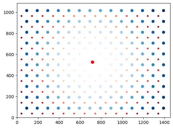
When calibrating at many points, we must be considerate of effects which are not present in single-point calibration. Specifically, each calibration point has a -1th order mirror in addition to the target 1st order location. These -1th orders act as noise for the other points. However, careful choice of how the grid of calibration points is aligned can lead to these mirror images avoiding sensitive regions. This is handled automatically by .wavefront_calibration_points(). In the below plot,
the red spots are mirror images of the blue spots, with the intensity corresponding to the spot index.
[5]:
points_ij = fs.wavefront_calibration_points(100, avoid_mirrors=True, plot=True);
Multipoint Superpixel Wavefront Calibration#
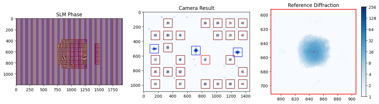
To start, we explore an extension to superpixel-based calibration where we calibrate many points simultaneously. Using the calibration_points=None, the field of view is densely packed with interference regions which are of appropriate size and of sufficient separation for the given superpixel_size.
[7]:
cam.set_exposure(.1)
movie = fs.wavefront_calibrate_superpixel(
    calibration_points=None,
    field_point=(.25, 0),
    field_point_units="freq",
    superpixel_size=75,
    test_index=2,                       # Testing mode
    phase_steps=10,
    plot=3                              # Special mode to generate a phase .gif
)

from slmsuite.holography.analysis.files import write_image

write_image("wavefront-simutaneous.gif", movie)

We use markdown to display the .gif we just made:
Some of the calibration points are not measured during this frame because there is a conflict with another pair. There’s a complex scheduling algorithm running in the background to make sure all pairs of reference and target superpixels are measured despite these conflicts.
Next, we can perform the calibration.
[13]:
cam.set_exposure(.1)
fs.wavefront_calibrate_superpixel(
    calibration_points=None,
    field_point=(.25, 0),
    field_point_units="freq",
    superpixel_size=75,
);
The longer runtime is slightly due to scheduling against conflicting superpositions positions, but mainly due to the overhead of fitting many 2D sinc terms every iteration. Future optimizations could bring this down to 30 minutes or so.
[14]:
fs.write_calibration("wavefront_superpixel")
[14]:
'C:\\Users\\Experiment\\Documents\\GitHub\\slmsuite-examples\\examples\\02C5V-2018021001-wavefront_superpixel-calibration_00002.h5'
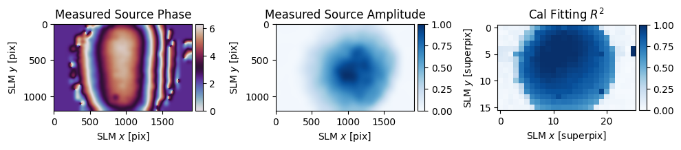
We can use a helper function _wavefront_calibration_superpixel_plot_raw() to see what we got. In our case, the calibrations points at the corners of our field of view have indices [44, 43, 36, 34].
[65]:
for i in [44, 43, 36, 34]:
    fs._wavefront_calibration_superpixel_plot_raw(index=i, r2_threshold=.5);
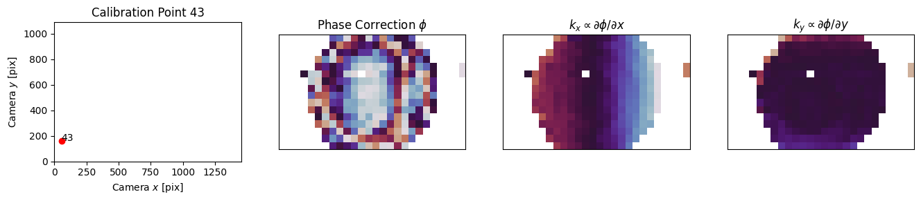
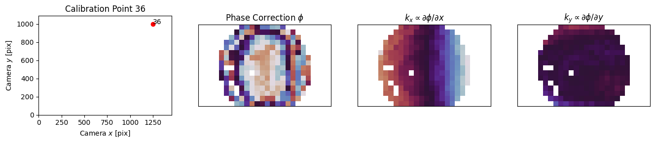
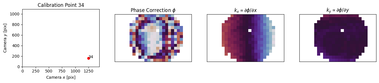
This above helper function is currently private and hidden because the analysis routines for this full-field calibration are not yet finalized. However, the analysis and smoothing for single-point calibration can still be run by again selecting the proper index. We don’t (currently) have a way to simulate varying aberration across the field of view, so if you’re running virtual hardware you will observe the same aberration at each point.
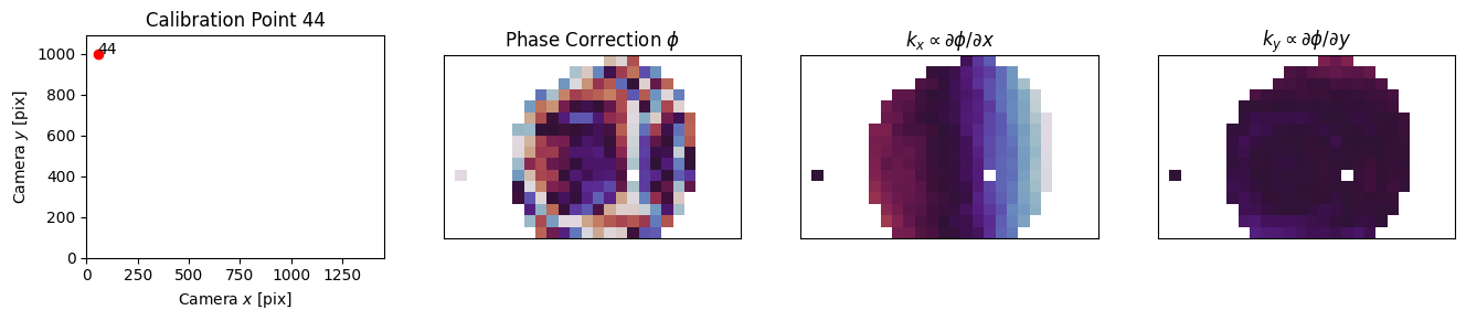
[60]:
phases = []
for i in [44, 43, 36, 34]:
    dat = fs.wavefront_calibration_superpixel_process(index=i, r2_threshold=.5, smooth=True, plot=True);
    phases.append(dat["phase"])
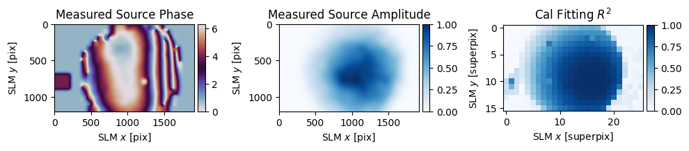
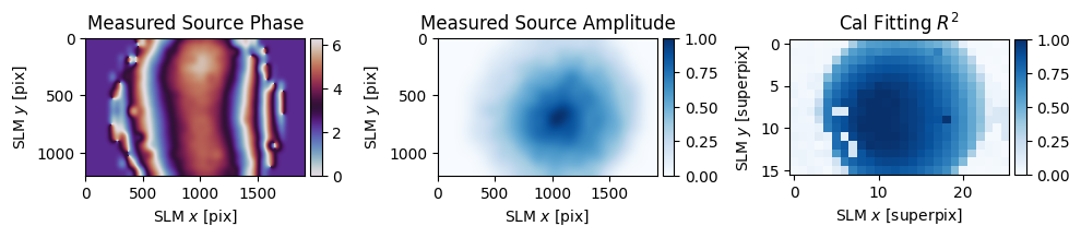
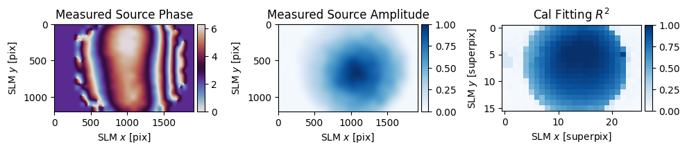
In our simple setup, most of the aberration comes from the SLM itself, but most of the spatially-varying aberration likely comes from the single 150 mm achromatic lens which separates the SLM from the camera. Even in this very simple setup, we observe order 1 wave (\(2\pi\)) of aberration differece across the field of view.
[66]:
slm.plot(phases[1] - phases[2]);
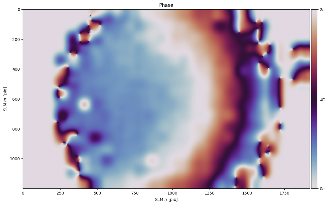
This problem is exacerbated for high-NA setups where light is bent to a much larger degree than our simple <.1 NA setup does. As field of view sizes are pushed larger and larger, our software solution to compensating for aberration becomes increasingly important to close the gap between imperfect aberration mitigation engineered into the optical train and the ideal of aberration-free imaging.
Zernike Wavefront Calibration#
With extent of the varying aberration established with the superpixel approach, we can turn our attention to a faster (and arguable more direct) way to compensate for aberration across many spots. Let’s start by removing the phase calibration applied to the SLM in the previous section so we can work from the start without correction.
[ ]:
if "phase" in slm.source: del slm.source["phase"]
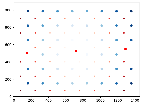
We can make use of the Zernike spot optimization explored in the previous example to directly and iteratively remove aberration from every spot. The function .wavefront_calibrate_zernike() accepts vectors in Zernike-space, such that the user can provide an arbitrary set of points to correct or further-correct. We first need to build these vectors from camera coordinates.
[5]:
from slmsuite.holography.toolbox import convert_vector

points_ij = fs.wavefront_calibration_points(100)

points_zernike = convert_vector(
    points_ij,
    from_units="ij",
    to_units="zernike",
    hardware=fs
)
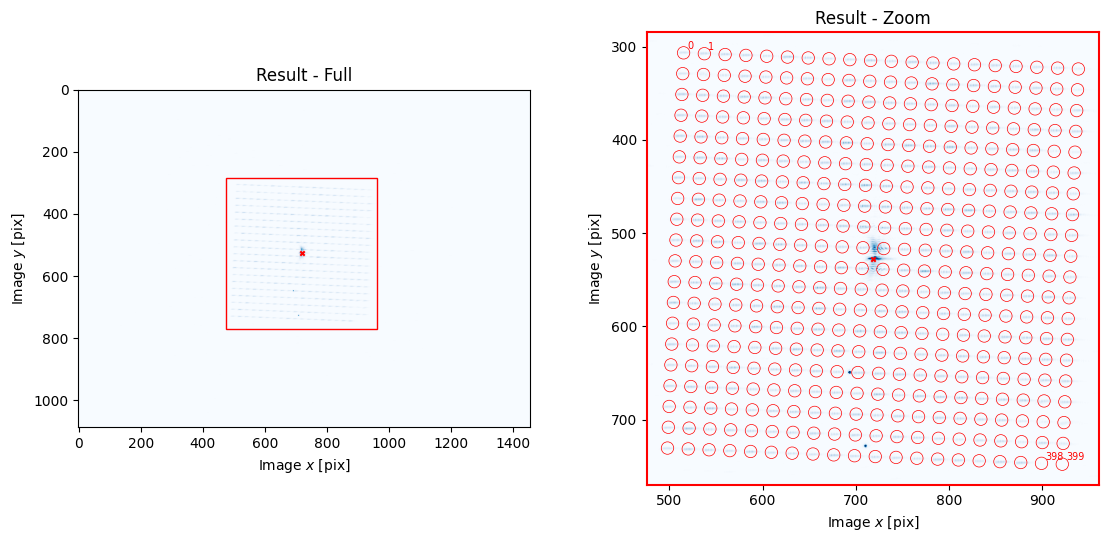
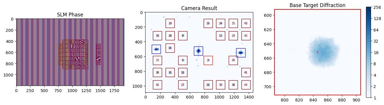
We can test the Zernike wavefront calibration settings by settings perturbation=0 (no iterative Zernike perturbation).
[6]:
cam.set_exposure(.02)
fs.wavefront_calibrate_zernike(points_zernike, perturbation=0, plot=True)
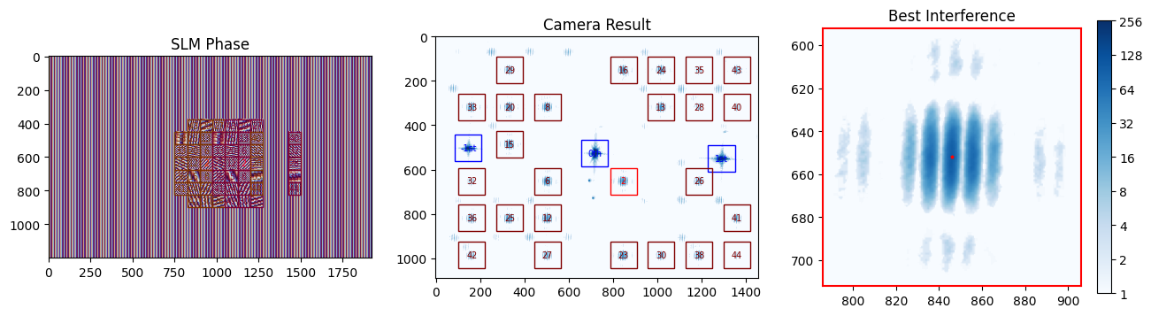
Now let’s actually run the calibration. The zernike_indices= argument allows the user to either say what the desired Zernike basis is or ask for a number of (non-piston) Zernike terms. The 2D vectors that we’re providing is assumed to be the \(x,y\) terms and the vectors are zero-padded to include another 7 terms in Zernike-space, for the 9 indices that we request.
The perturbation= argument determines the size of our sweep in radians. For the current code, using a smallish perturbation and iterating seems to work best, so we will do this.
[7]:
fs.wavefront_calibrate_zernike(points_zernike, zernike_indices=9, perturbation=1, plot=True);

Passing None in place of the points tells .wavefront_calibrate_zernike() to use the result of the previous calibration, so this is an easy way to iterate the calibration. Let’s do a few more iterations (but forego the plots except for on the last one):
[8]:
N = 4

for i in range(N):
    fs.wavefront_calibrate_zernike(None, zernike_indices=9, perturbation=1, plot=(i == N-1))

The optimization currently takes several iterations, in part because of imperfect orthonormality of the Zernike terms. What we want to see (and do see) is stability in the convergence at the end of the optimization. We see stability to around <.2 radians, or about 30 miliwaves per term. Virtual hardware is able to get to <.1 radians fairly easily. Additionally, having a decent guess of the initial aberration, whether by Zernike fit to the superpixel wavefront calibration or fastphase, can
help the optimization to find an early minimum.
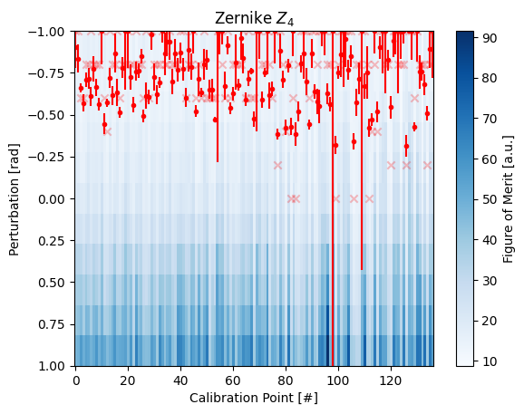
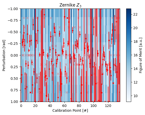
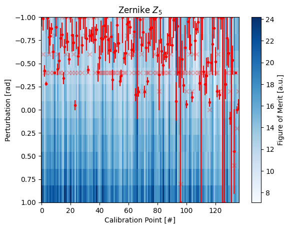
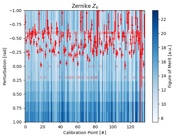
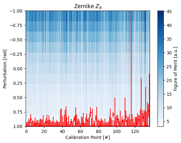
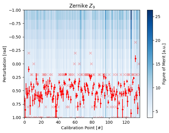
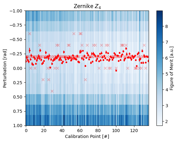
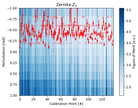
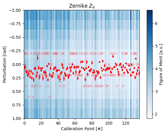
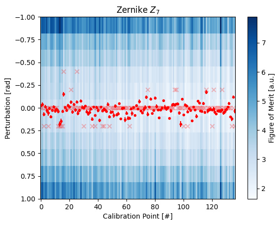
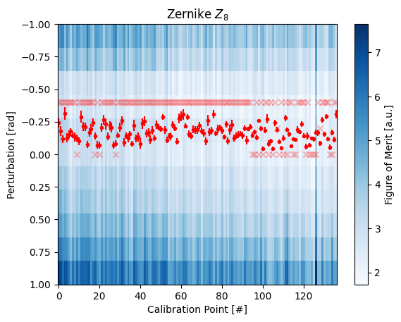
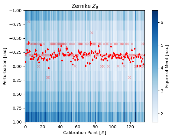
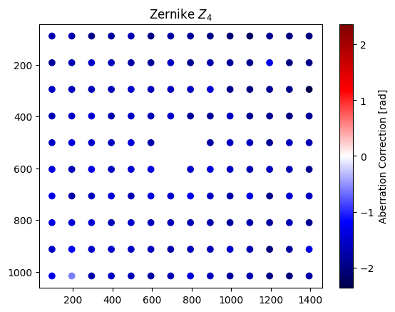
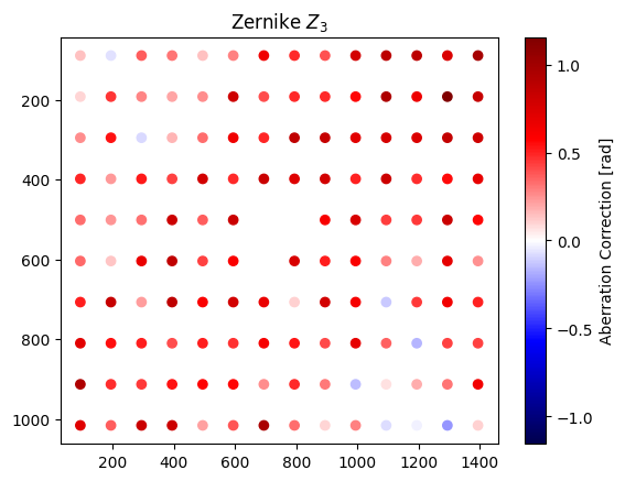
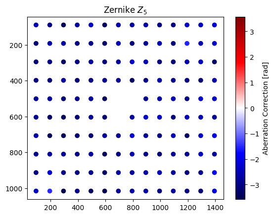
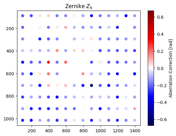
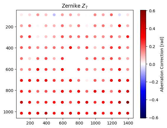
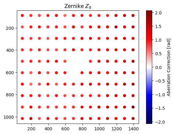
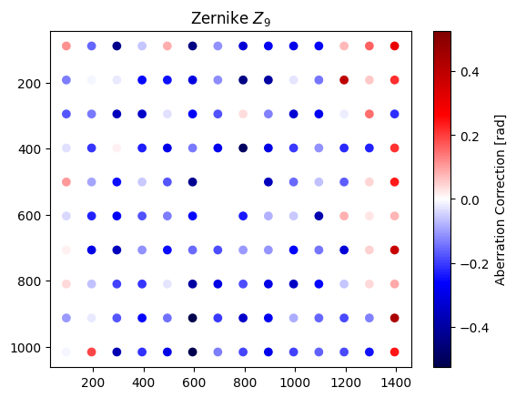
We can take a look at the final results by plotting the data directly:
[9]:
for index in range(2,9):
    fs.wavefront_calibrate_zernike_plot_raw(index)
    plt.show()
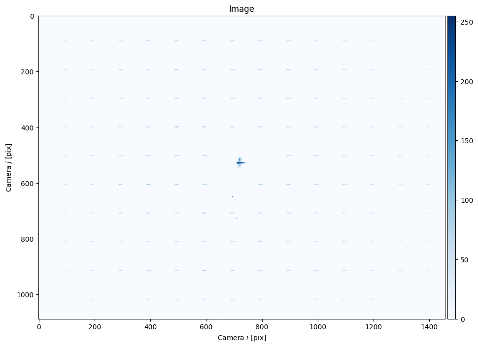
We can also examine the image directly, by again using perturbation=0 as a proxy:
[10]:
fs.wavefront_calibrate_zernike(None, zernike_indices=9, perturbation=0, plot=True)

Nice, tight spots.
It’s also important to mention that this method is extremely general. .wavefront_calibrate_zernike() accepts user-provided functions to change the metric= of how spot images from the camera are judged, or completely change the heuristic by providing a custom callback=.
The
metric()takes in a stack of spot images, each image corresponding to one spot, and is respected to return a list of the goodness of each image.callback()overrides camera functionality and the user can choose how to determine the goodness. This, for instance, could be a measure of trap depth on atoms or similar measurement that avoids aberration between the camera and an experimental plane. After all, perfect spots on the camera might correspond to very distorted spots in an experimental plane.
Future additions to slmsuite will take greater advantage of this full-field calibration information. We look forward to seeing how far we can push this frontier!