

Zernike Holography#
Optical aberration is a pervasive roadblock to good imaging. Aberration can be modeled as a phase distortion upon an optical wavefront: while a flat wavefront is free of aberration, non-ideal optical elements impart a sort of distortion hologram on the beam leading to distorted spots. Zernike polynomials act as a good (orthonormal under some conditions) basis to describe optical aberration, with terms corresponding directly to common forms of aberration.
We have already investigated simple wavefront calibration in a previous example. The action of this calibration is (in part) to measure the phase distortion and then compensate for the known distortion by subtracting the phase from the phase of desired holograms. However, a major problem with this technique is that the measured phase is only valid for the \(k\)-vector (corresponding to a point on the camera) at which the calibration was measured. Other \(k\)-vectors (points across the
field of view of the camera) experience a different optical path through the optical train and thus experience a different aberration. In systems with strong distortion, this can lead to good sharp wavefront correction only in the neighborhood surrounding the calibration point such as seen in slmsuite issue #30.
This phenomenon is an invarient for additive correction; one cannot find a single addative correction mask to correct all \(k\)-vectors for a given hologram. The solution is to instead “bake” the correction into the hologram itself. In the case of spot holograms, instead of thinking of mapping power to points in 2D space, it is instead more practical to think of mapping power to points in Zernike aberration space, where each spot has a unique Zernike calibration.
Initialization#
To start, we initialize our system:
[3]:
slm = Santec(slm_number=1, display_number=2, wav_um=.633, settle_time_s=.5); print()
cam = AlliedVision(serial="02C5V", pitch_um=(3.45, 3.45), fliplr=True)
fs = FourierSLM(cam, slm)
Santec slm_number=1 initializing... success
Looking for display_number=2... success
Opening LCOS-SLM,SOC,8001,2018021001... success

vimba initializing... success
Looking for cameras... success
vimba sn '02C5V' initializing... success
[4]:
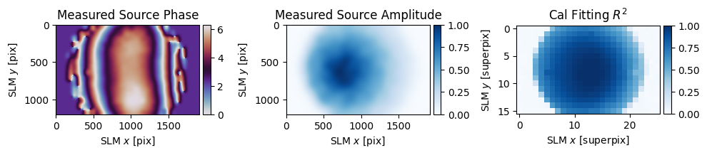
fs.read_calibration("wavefront_superpixel")
fs.wavefront_calibration_superpixel_process(r2_threshold=.5, plot=True);
[5]:
cam.set_exposure(.002)
fs.fourier_calibrate(20, 20, plot=True)
[5]:
{'M': array([[28857.04043148, -1177.85636476],
        [ 1180.05882475, 28860.25741903]]),
 'b': array([[722.91543747],
        [527.53302081]]),
 'a': array([[-8.76122968e-21],
        [ 5.60718699e-19]]),
 '__version__': '0.1.0',
 '__time__': '2024-07-26 00:56:16.348606',
 '__timestamp__': 1721969776.348606,
 '__meta__': {'camera': '02C5V', 'slm': '2018021001'}}
Zernike Indexing#
There are many ways to index Zernike polynomials. slmsuite supports a number of conventions, but uses the 1D ANSI "ansi" indexing \(i\) as the default. We can find the mapping \(Z_i = Z_n^l\) between ANSI and the canonical definition "radial" consisting of the radial \(n\) and azimuthal \(l\) orders:
[6]:
from slmsuite.holography.toolbox.phase import zernike_convert_index

ansi = np.arange(10)
radial = zernike_convert_index(ansi, from_index="ansi", to_index="radial")
print(radial)
[[ 0  0]
 [ 1 -1]
 [ 1  1]
 [ 2 -2]
 [ 2  0]
 [ 2  2]
 [ 3 -3]
 [ 3 -1]
 [ 3  1]
 [ 3  3]]
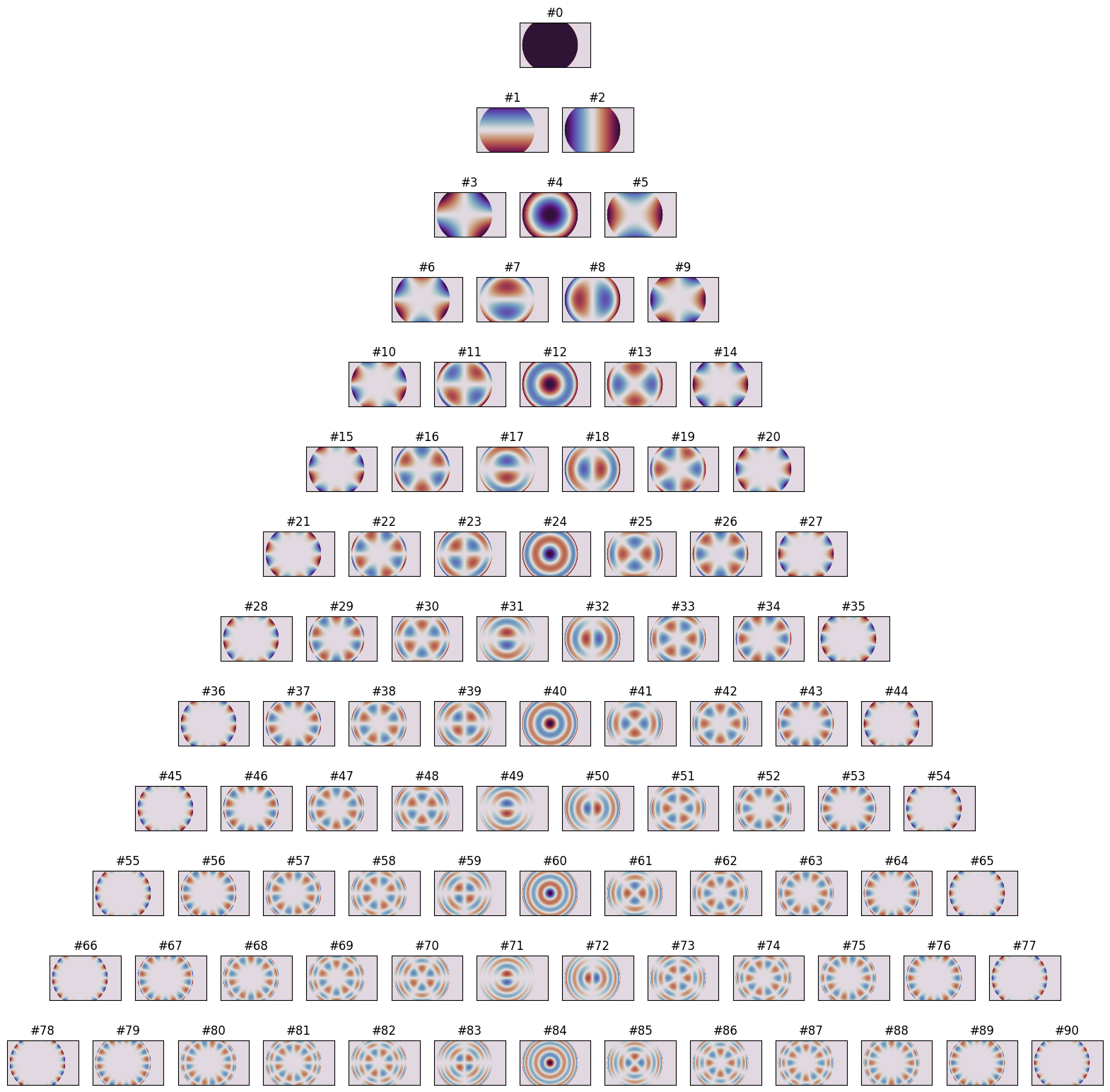
The nature of the radial \(n\) and azimuthal \(l\) orders make it often convenient to arange the polynomials in a pyramid:
[7]:
from slmsuite.holography.toolbox.phase import zernike_pyramid_plot

plt.figure(figsize=(20,20))
zernike_pyramid_plot(slm, order=3)
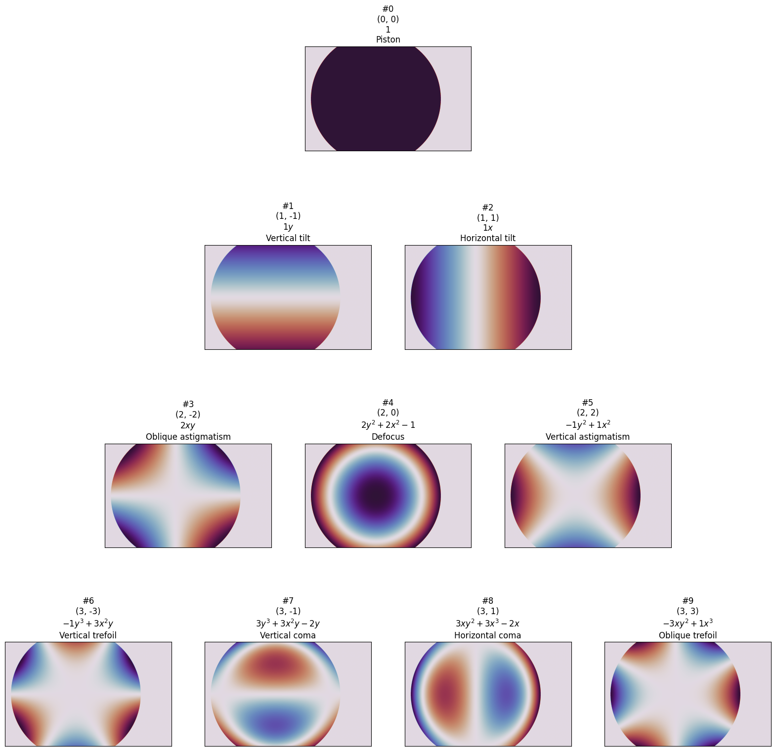
Notice how the polynomials are translated and scaled to correspond with the measured amplitude distribution of the SLM. This is because slmsuite is automatically computing the best center point and scaling radius for the polynomials based upon fitting to the measured amplitude distribution. This allows the Zernike basis to act accurately upon the spot, without laterally steering the beam while focusing, for instance.
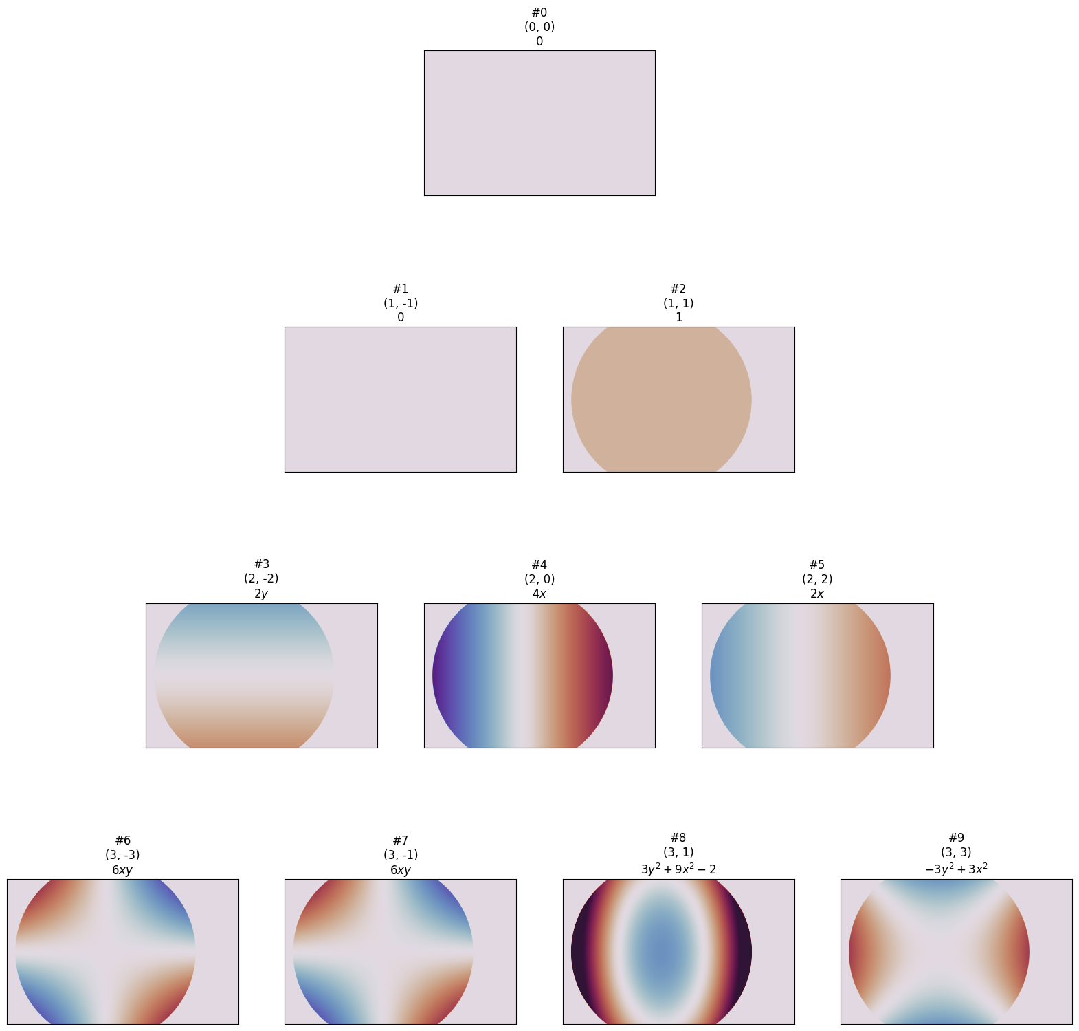
slmsuite also supports derivates (computed analyticaly via the power rule before rendering, for speed):
[8]:
plt.figure(figsize=(20,20))
zernike_pyramid_plot(slm, order=3, derivative=(1, 0), scale=5)    # Adjust the scale because the derivative exceeds [-1, 1]
We can do this for very high order \(n\):
[9]:
from slmsuite.holography.toolbox.phase import zernike_pyramid_plot

plt.figure(figsize=(20,20))
zernike_pyramid_plot(slm, order=12, titles=["ansi"])
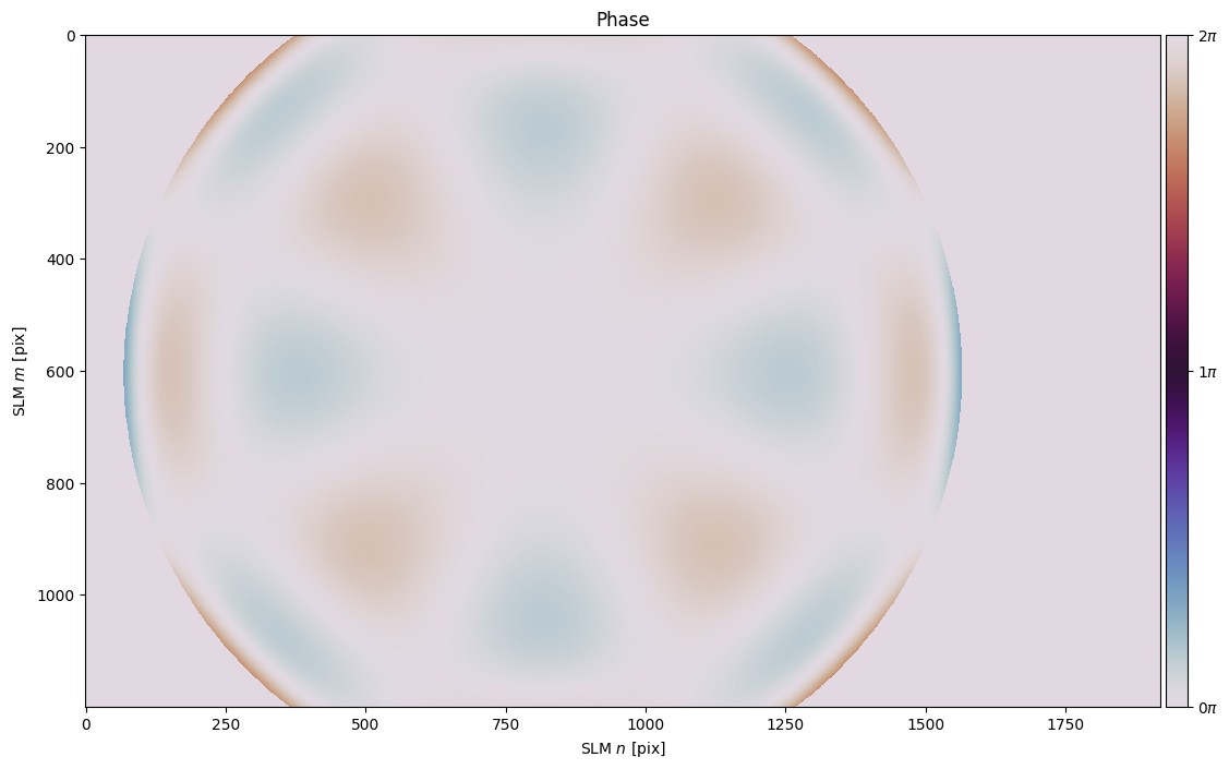
To actually grab the phase of a single polynomial, we can use zernike(). This is of the same style as other functions in toolbox.phase, where the SLM is passed as grid= to give the function information about the scaling of the polynomial.
[10]:
from slmsuite.holography.toolbox.phase import zernike

zernke_42 = zernike(slm, 42)

slm.plot(zernke_42);
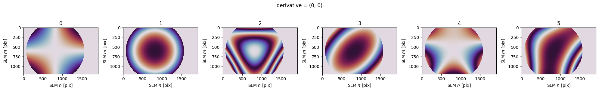
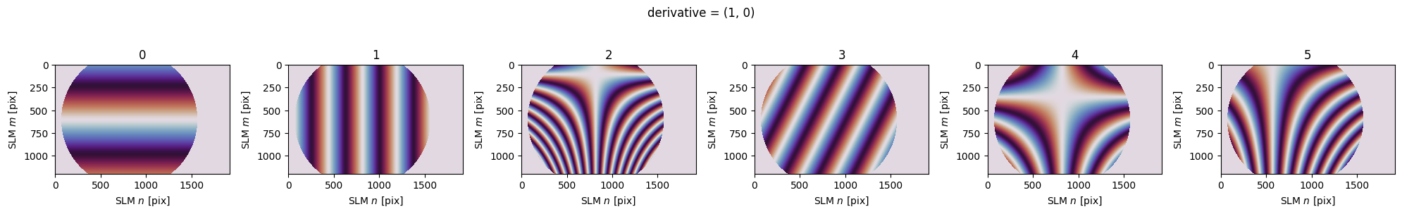
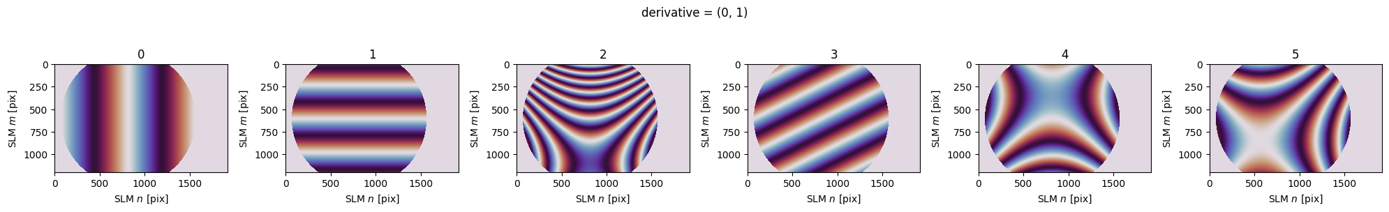
The core function zernike_sum() supports generating stacks of sums of Zernike polynomials, with derivatives are applied to each. The weights= term is here a (4, 6) matrix, 4 terms for the requested ANSI indices, 6 terms for the 6 produced sums. These weights \(w_i^{(j)}\) are multiplied directly with \(Z_i\) (normalized to \(\pm 1\)), to produce \(\phi_j = \sum_j w_i^{(j)}Z_i\).
[11]:
for derivative in [(0,0), (1,0), (0,1)]:
    images = np.pi * zernike_sum(
        slm,
        indices=[3,4,5,6],
        weights=[
            [1,0,0,1,0,1],      # 3
            [0,1,2,1,0,1],      # 4
            [0,0,0,0,1,1],      # 5
            [0,0,2,0,1,1],      # 6
        ],
        derivative=derivative
    )

    fig, axs = plt.subplots(1, 6, figsize=(20,3))

    for i, image in enumerate(images):
        plt.sca(axs[i])
        slm.plot(image, title=str(i), cbar=False)

    plt.suptitle(f"derivative = {derivative}")
    plt.tight_layout()
    plt.show()
3D “Compressed Spot” Holography#
3D spots is a first simple application of the math which “bakes” aberration into a hologram. Indeed, the \(Z_4 = Z_2^0\) Zernike polynomial is exactly defocus, and it is this parabolic term which we will use for translating (aberrating) in \(z\). Our previous examples effectively only used the \(x = Z_2 = Z_1^1\) and \(y = Z_1 = Z_1^{-1}\) terms.
Let’s start by making a desired pointcloud in the camera’s pixel "ij" coordinates.
[12]:
from slmsuite.holography.toolbox import convert_vector

N = 100
x = np.arange(N) / 20

zeroth_order_ij = convert_vector((0,0), from_units="norm", to_units="ij", hardware=fs)

vectors_ij = np.vstack((
    50 * (x + 1) * np.cos(2 * np.pi * x) + zeroth_order_ij[0],
    50 * (x + 1) * np.sin(2 * np.pi * x) + zeroth_order_ij[1],
    200 * np.cos(1.5 * np.pi * x)
))
Unit conversions is a major focus of slmsuite. The core method toolbox.convert_vector() described previously supports 3D points and converts between the various units. For most units, “focal power” \(1/f\) is used for \(z\), but with Fourier calibration and knowledge of the camera’s pixel pitch in microns, this extends to true cartesian vectors. If you don’t have the .pitch_um parameter of the camera set, you will probably see nan for all the \(z\) coordinates except
for "ij".
[13]:
from slmsuite.holography.toolbox import print_blaze_conversions

print_blaze_conversions(
    vectors_ij[:, 0],       # Print the first vector.
    from_units="ij",
    hardware=fs,
    shape=(2048, 2048)
)
'rad' : [ 1.72979248e-03 -7.07289906e-05  4.39884247e-08]
'mrad' : [ 1.72979248e+00 -7.07289906e-02  4.39884247e-08]
'deg' : [ 9.91098083e-02 -4.05247265e-03  4.39884247e-08]
'norm' : [ 1.72979248e-03 -7.07289906e-05  4.39884247e-08]
'kxy' : [ 1.72979248e-03 -7.07289906e-05  4.39884247e-08]
'knm' : [1.06877239e+03 1.02216931e+03 4.39884247e-08]
'freq' : [ 2.18615163e-02 -8.93889297e-04  4.39884247e-08]
'lpmm' : [ 2.73268954e+00 -1.11736162e-01  4.39884247e-08]
'zernike' : [102.79924314  -4.2033289    6.18145023]
'ij' : [772.91543747 527.53302081 200.        ]
'm' : [0.00266656 0.00181999 0.00069   ]
'cm' : [0.26665583 0.18199889 0.069     ]
'mm' : [2.66655826 1.81998892 0.69      ]
'um' : [2666.55825928 1819.98892179  690.        ]
'nm' : [2666558.25928285 1819988.92178871  690000.        ]
'mag_m' : [0.00266656 0.00181999 0.00069   ]
'mag_cm' : [0.26665583 0.18199889 0.069     ]
'mag_mm' : [2.66655826 1.81998892 0.69      ]
'mag_um' : [2666.55825928 1819.98892179  690.        ]
'mag_nm' : [2666558.25928285 1819988.92178871  690000.        ]
The "zernike" conversion is listed as the coefficients (in radians) of the \(Z_2, Z_1, Z_4\) terms, which correspond to \(x,y,z\), the tilt and focus terms (see the pyramid).
We can now make the hologram with these 3D points.
[14]:
from slmsuite.holography.algorithms import CompressedSpotHologram

hologram = CompressedSpotHologram(
    spot_vectors=vectors_ij,
    basis="ij",                 # For 3D spots, the basis defaults to Zernike terms [2,1,4] = [x,y,z].
    cameraslm=fs
)
hologram.optimize()
In the future, this example will be updated to describe how this process for “compressed” holography actually works. In the meantime, let’s take a look at what we made:
[15]:
hologram.plot_farfield(limit_padding=-.4);
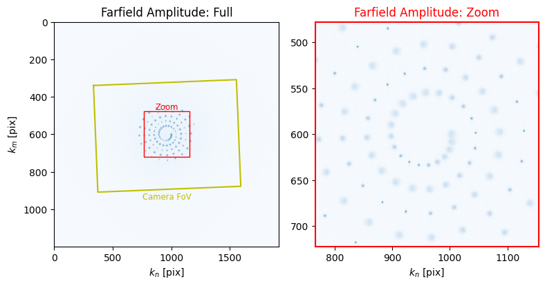
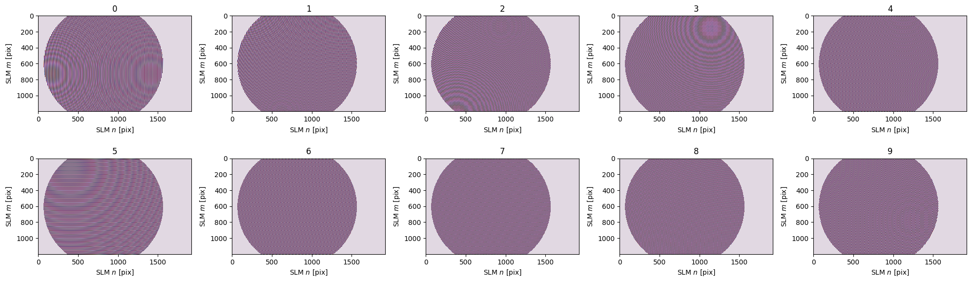
Under the hood, slmsuite is using the cached conversion and convert_vector() to translate the "ij" coordinates into to "zernike" space and make a basis of “compressed kernels” which map to each spot in this three-dimensional aberration space. We can look at this basis of Zernike polynomial kernels (only plotting the first ten for speed) by feeding the vector in aberration space as weights= of zernike_sum().
[16]:
# Get the coordinates in "Zernike space" using the [2,1,4] = [x,y,z] terms.
vectors_zernike = convert_vector(
    vectors_ij,
    from_units="ij",
    to_units="zernike",
    hardware=fs
)

# Plot only the first 10.
images = np.pi * zernike_sum(
    slm,
    indices=None,       # For 3D spots, the basis defaults to Zernike terms [2,1,4].
    weights=vectors_zernike[:, :10]
)

fig, axs = plt.subplots(2, 5, figsize=(20,6))
axs = axs.ravel()

for i, image in enumerate(images):
    plt.sca(axs[i])
    slm.plot(image, title=str(i), cbar=False)

plt.tight_layout()
plt.show()
[ ]:
Zernike Spot Holography#
However, this technique is extensible to far more than the three \(Z_2, Z_1, Z_4\) terms. Let’s make a realized Zernike pyramid in a single hologram.
First, let’s find the "zernike" coordinates of the pyramid corresponding to desired "ij" positions for arrangement according to the radial and azimuthal orders \(n\) and \(l\).
[17]:
from slmsuite.holography.toolbox import format_vectors

center = format_vectors((1000, 500))
res = (320, 320)
((i0, i1), (i2, i3)) = limits = (
    (int(center[0] - res[0]/2), int(center[0] + res[0]/2)),
    (int(center[1] - res[1]/2), int(center[1] + res[1]/2))
)

N = 28
i = np.arange(N)
nl = zernike_convert_index(i, from_index="ansi", to_index="radial")
ij = 20 * np.vstack((nl[:, 1], (3-nl[:, 0]) * np.sqrt(3))) + center
sz = convert_vector(ij, from_units="ij", to_units="zernike", hardware=fs)

plt.title("Zernike Basis Coordinates")
plt.scatter(sz[0], sz[1])
plt.gca().set_aspect("equal")

base = np.zeros((N,N))

base[2, :] = sz[0]      # Tilt x term
base[1, :] = sz[1]      # Tilt y term

We impart the Zernike term for each spot by adding a perturbation in Zernike-space, which we have requested to be \(N\)-dimensional; one order for each spot. The second and third rows correspond to the steering to position the spot at the correct \(n,l\) coordinate in the pyramid in 2D space, according to the \(y = Z_1\) and \(x = Z_2\) terms. Imparting the perturbation for \(Z_i\) on the correct spot at the correct \(n,l\) coordinate is as simple as adding an identity matrix. Then, the \(i\)th spot is given the perturbation for \(Z_i\):
[18]:
perturbation = np.diag(np.ones(N))
print((base + 10*perturbation)[:10, :10].astype(int))
[[ 10   0   0   0   0   0   0   0   0   0]
 [133  74  60  -5  -8 -12 -74 -78 -81 -84]
 [576 532 624 488 570 652 444 526 608 690]
 [  0   0   0  10   0   0   0   0   0   0]
 [  0   0   0   0  10   0   0   0   0   0]
 [  0   0   0   0   0  10   0   0   0   0]
 [  0   0   0   0   0   0  10   0   0   0]
 [  0   0   0   0   0   0   0  10   0   0]
 [  0   0   0   0   0   0   0   0  10   0]
 [  0   0   0   0   0   0   0   0   0  10]]
Then, we send these desired coordinates to optimization:
[24]:
hologram = CompressedSpotHologram(
    spot_vectors=base + 5*perturbation,
    basis=i,
    cameraslm=fs
)

hologram.optimize()
Let’s see what we got:
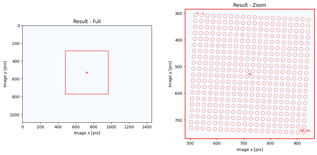
[27]:
slm.write(hologram.get_phase())
cam.set_exposure(.008)
cam.flush()
cam.plot(limits=limits, title="Realized Zernike Pyramid");
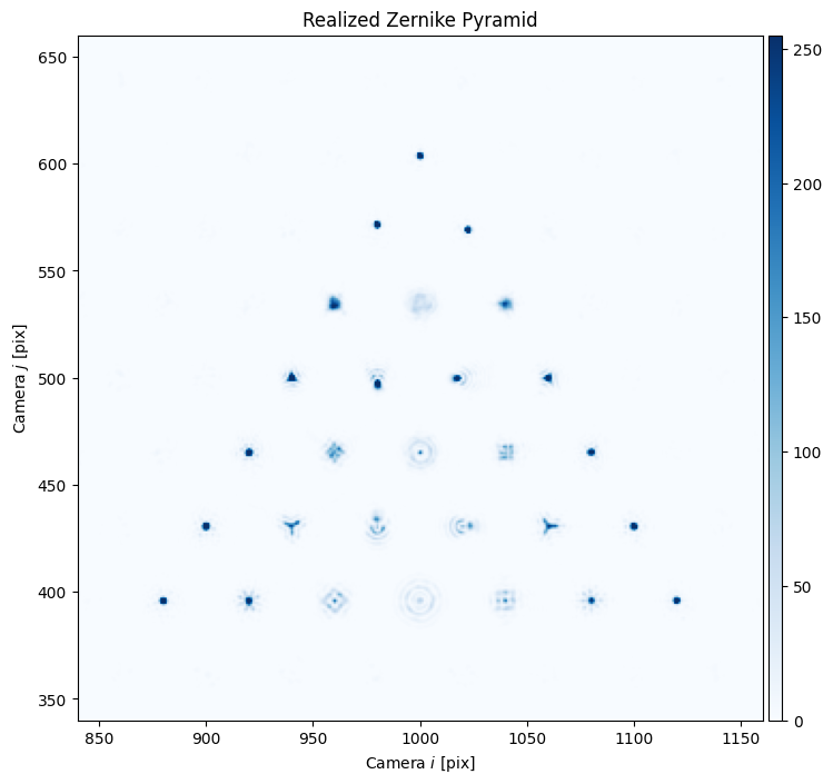
This result looks even cleaner with virtual holography, but our real source distribution isn’t a perfect Gaussian on our physical SLM.
To show how programmable this technique of targeting points in Zernike-space is, we make a fun .gif, modulating the level of perturbation:
[30]:
import tqdm.auto as tqdm

# Make the hologram
hologram = CompressedSpotHologram(
    spot_vectors=base,
    basis=i,
    cameraslm=fs
)
hologram.optimize("WGS-Leonardo", maxiter=50, verbose=False)

# Build the term osillation movie.
imgs = []
X = 5 * np.sin(np.linspace(0, 2*np.pi, 25, endpoint=False))

cam.set_exposure(.004)

for x in tqdm.tqdm(X):
    # Optimize to the new position.
    hologram.spot_zernike = base + x*perturbation
    hologram.optimize("WGS-Leonardo", maxiter=20, verbose=False)

    # Project the pattern.
    slm.write(hologram.get_phase())
    cam.flush()
    imgs.append(cam.get_image()[i3:i2:-1, i0:i1])
(We use a helper function to render stored raw data with colormaps, saving the stack of images as a .gif):
[31]:
from slmsuite.holography.analysis.files import write_image

imgs2 = np.array(imgs, copy=True)
imgs2[imgs2 > 127] = 127
imgs2 *= 2

write_image("ex-zernike-spots.gif", imgs2, cmap="Blues", border=127, normalize=False)
write_image("ex-zernike-spots-dark.gif", imgs, cmap="turbo", border=127, normalize=False)
This feature is be applied to wavefront calibration in the next example, to transcend the spatial dependence of aberration across a field of view.
[ ]: