Simulation
Even in the absence of an experimental setup, slmsuite is an ideal testbed for new holography algorithms and SLM techniques. Here, we demonstrate the basic simulation features of slmsuite to investigate the accuracy of the package’s wavefront calibration routines.
Simulated SLMs
SimulatedSLM is a testbed for implementing physical non-idealities of spatial light modulators, including panel curvature (near-field phase distortions), cross-talk/mutual coupling, and non-uniform control value-to-phase shift transduction across the aperture.
We start by building a SimulatedSLM with an arbitary flatness map (using slmsuite’s Zernike functions) and elliptical source illumination.
[2]:
from slmsuite.hardware.slms.simulated import SimulatedSLM

# SLM resolution in pixels
res = (640,480)
bits = 8

#Build an arbitrary flatness map
dummy_slm = SimulatedSLM(res)
phase_abberation = toolbox.phase.zernike_sum(dummy_slm,
    weights=(((2, 0),  7),       # Z_20
             ((2, 1), -8),       # Z_21
             ((3, 1),  9)),      # Z_31
    aperture="cropped")

# The abberated SLM
slm = SimulatedSLM(res, bitdepth=bits)
slm.set_source_analytic('gaussian2d', x0=0, y0=0, a=1, c=0, wx=0.4, wy=0.3, units="frac",
                         phase_offset = phase_abberation,
                         sim = True)
slm.plot_source(sim=True);
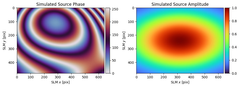
SimulatedSLM’s (simulated) source attribute is independent of the SLM phase attribute, and is applied whenever phase is written to the SLM. We can therefore see the true phase profile of the SLM by plotting the display attribute.
Simulated Cameras
SimulatedCam computes the far-field of SimulatedSLM with desired imaging transformations.
[3]:
from slmsuite.hardware.cameras.simulated import SimulatedCam

# Option 1: demonstrate the full capability of the simulation mode.
# The simulated camera computes images projected by `slm` with the desired
# affine transformation and noise. Computing the intensity at each
# camera pixel therefore requires (slow) interpolation from the computed
# (and heavily padded) SLM far-field.
# Note that f_eff is in units pix/radian by default.
# Since the max steering angle is O(1 rad), f_eff~slm_res is a good proxy for unity magnification.

cam_res = (512,512)
cam_bits = 14 # Since camera precision typically limits convergence, we'll simulate a low-quanization-noise unit.
# readout_noise = {'read': lambda img: np.random.poisson(0.01*img)} # Support for readout noise & dark current
cam = SimulatedCam(slm, cam_res, bitdepth=cam_bits)
cam.set_affine(f_eff=1.2*res[0], theta=np.pi/10)

# Option 2: fastest simulation.
# Directly sample the SLM far-field without transformations since the
# "ij" and "knm" bases are equivalent.

# cam = SimulatedCam(slm)
Padded SLM k-space shape set to (1024,1024) to achieve required imaging resolution.
Padded SLM k-space shape set to (1024,1024) to achieve required imaging resolution.
C:\Users\Experiment\Documents\GitHub\slmsuite\docs\slmsuite-examples\examples\../../..\slmsuite\hardware\cameras\simulated.py:189: UserWarning: Camera extends beyond the accessible SLM k-space; some pixels may not be targetable.
  warnings.warn(
Also note that since we created this simulated camera without specifying the effective focal length \(f_\text{eff}\) between the SLM and camera, slmsuite computed the minimum effective focal length \(f_\text{min}\) that places the camera fully within the SLM’s accesible \(k\)-space. For more notes on \(f_\text{eff}\) see the `SimulatedCam documentation <https://slmsuite.readthedocs.io/en/latest/_autosummary/slmsuite.hardware.cameras.simulated.html>`__.
[4]:
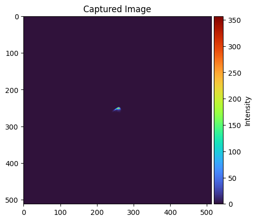
# Take a sample picture
im = cam.get_image(plot=True)
Using Simulation to Compare Wavefront Calibration Algorithms
Now that we have simulated SLM/camera pair, we can use slmsuite’s features normally, as if we had an experiment in hand! Here, we’ll use simulation mode to check the accuracy of various wavefront calibration techniques.
[5]:
fs = FourierSLM(cam, slm)
[6]:
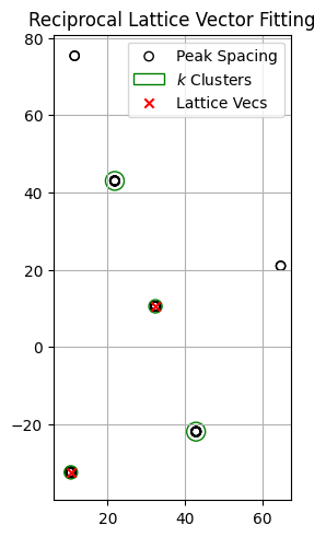
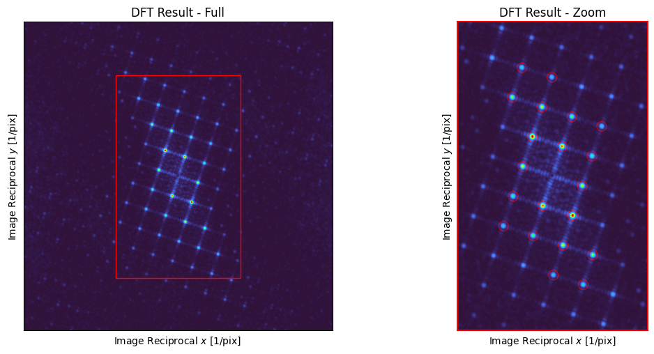
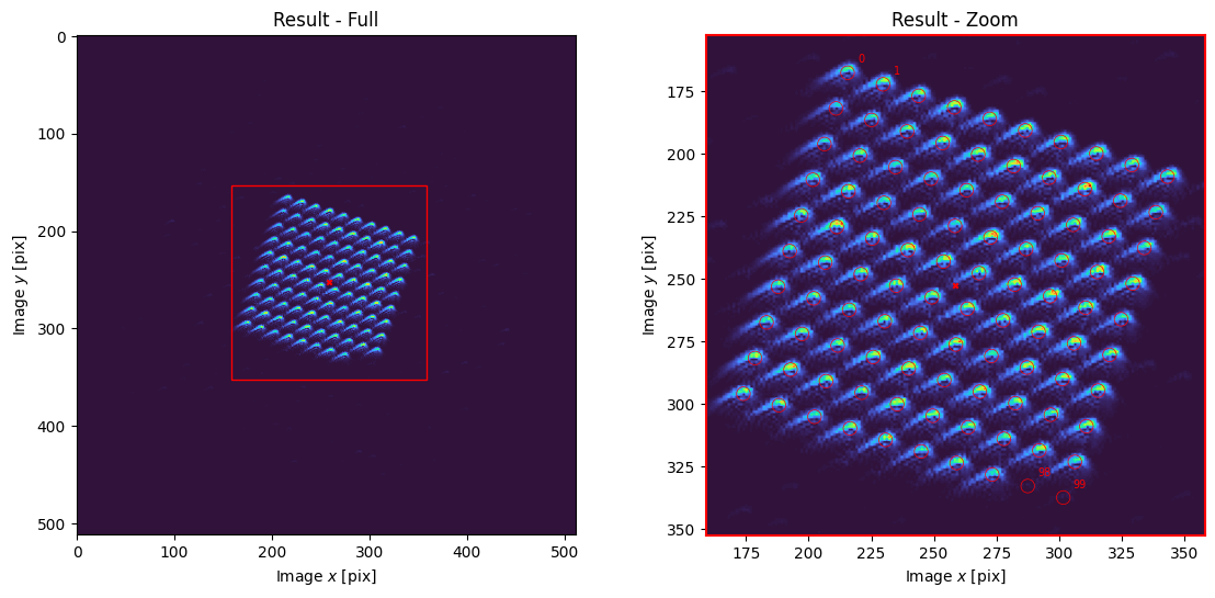
fs.fourier_calibrate(
    array_shape=[10, 10],           # Size of the calibration grid (Nx, Ny) [knm]
    array_pitch=[20, 20],           # Pitch of the calibration grid (x, y) [knm]
    autoexposure={"set_fraction":0.5},
    plot=True);
print(fs.fourier_calibration)
Reset exposure to 2.00s; maximum image value = 12.
Reset exposure to 4.00s; maximum image value = 24.
Reset exposure to 8.00s; maximum image value = 48.
Reset exposure to 16.00s; maximum image value = 96.
Reset exposure to 32.00s; maximum image value = 192.
Reset exposure to 64.00s; maximum image value = 383.
Reset exposure to 128.00s; maximum image value = 766.
Reset exposure to 256.00s; maximum image value = 1533.
Reset exposure to 512.00s; maximum image value = 3066.
Reset exposure to 1024.00s; maximum image value = 6131.
Reset exposure to 1368.23s; maximum image value = 8192.
{'M': array([[ 726.64901052, -236.60316689],
       [ 235.72750081,  728.72877373]]), 'b': array([[258.61784386],
       [252.54652068]]), 'a': array([[0.],
       [0.]])}
Once Fourier calibrated, we can wavefront calibrate. We’ll use phase_steps=1 first, which minimizes SLM writes by fitting the imaged 2D interference pattern between two superpixels. Let’s test a superpixel…
[7]:
fs.wavefront_calibrate(
    interference_point=(300, 300),
    field_point=(100, 100),
    field_point_units="ij",
    superpixel_size=40,
    phase_steps=1,
    test_superpixel=(4,4),
    plot=True,
    autoexposure=True);
C:\Users\Experiment\Documents\GitHub\slmsuite\docs\slmsuite-examples\examples\../../..\slmsuite\hardware\cameraslms.py:784: UserWarning: Non-resolvable interference fringe period for the given SLM calibration extent. Either exclude more of the SLM or magnify the field on the camera.
  warnings.warn(
Reset exposure to 2736.46s; maximum image value = 1012.
Reset exposure to 5472.91s; maximum image value = 2023.
Reset exposure to 10945.83s; maximum image value = 4047.
Reset exposure to 21891.65s; maximum image value = 8094.
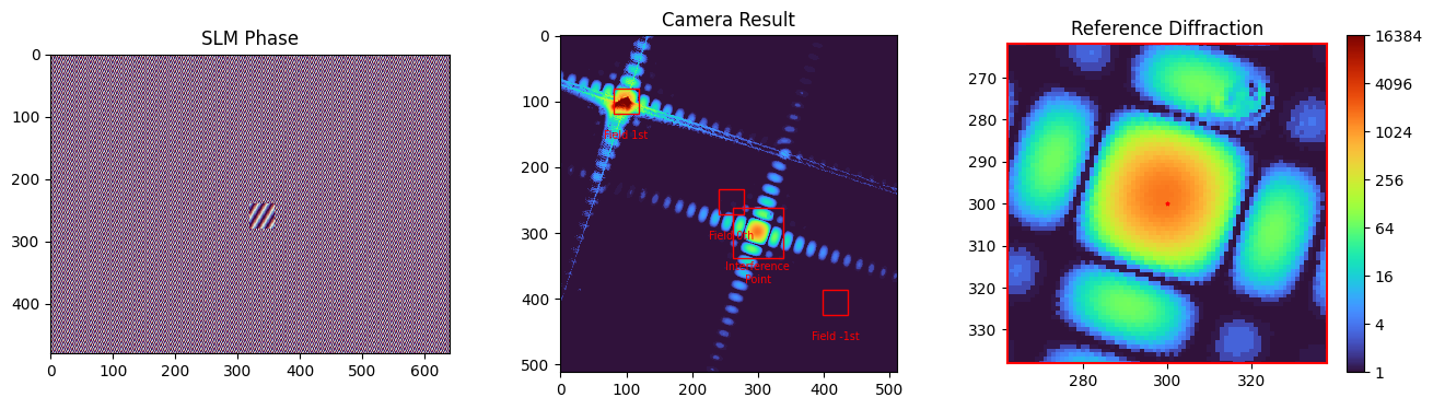
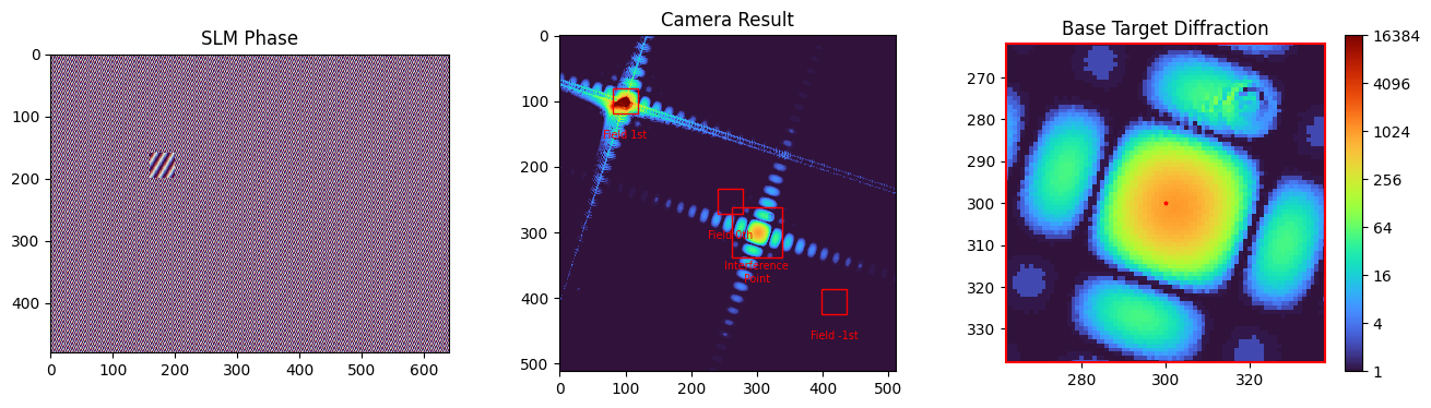
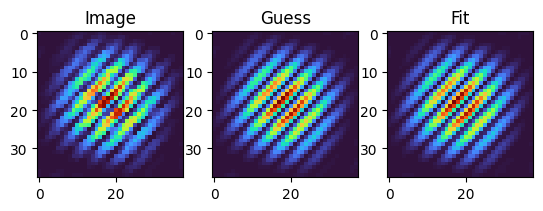
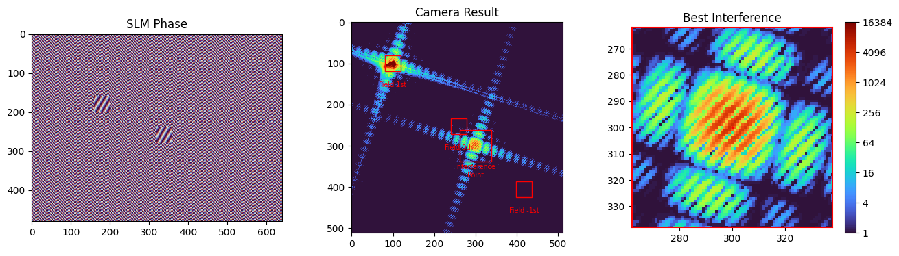
Looks good – let’s calibrate!
[8]:
fs.wavefront_calibrate(
    interference_point=(300, 300),
    field_point=(100, 100),
    field_point_units="ij",
    superpixel_size=40,
    phase_steps=1,
    plot=False,
    autoexposure=True);
Reset exposure to 8756.66s; maximum image value = 3238.
Reset exposure to 17513.32s; maximum image value = 6475.
Reset exposure to 22157.40s; maximum image value = 8192.
C:\Users\Experiment\Documents\GitHub\slmsuite\docs\slmsuite-examples\examples\../../..\slmsuite\hardware\cameraslms.py:1062: UserWarning: Image fitting failed; nulling response from this superpixel.
  warnings.warn("Image fitting failed; nulling response from this superpixel.")
C:\Users\Experiment\Documents\GitHub\slmsuite\docs\slmsuite-examples\examples\../../..\slmsuite\hardware\cameraslms.py:1068: RuntimeWarning: invalid value encountered in scalar divide
  contrast = np.abs(popt[1] / (np.abs(popt[1]) + np.abs(popt[3])))
C:\Users\Experiment\Documents\GitHub\slmsuite\docs\slmsuite-examples\examples\../../..\slmsuite\misc\fitfunctions.py:346: RuntimeWarning: divide by zero encountered in scalar divide
  return np.square(np.sinc((1 / R) * x) * np.sinc((1 / R) * y)) \
C:\ProgramData\Anaconda3\envs\slmsuite\Lib\site-packages\numpy\lib\function_base.py:3639: RuntimeWarning: invalid value encountered in sin
  return sin(y)/y
[9]:
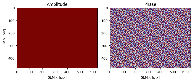
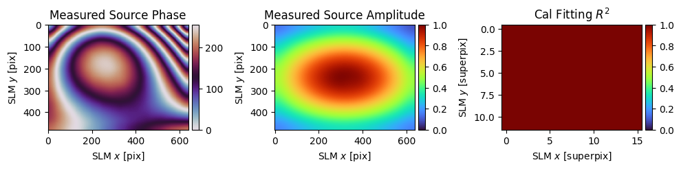
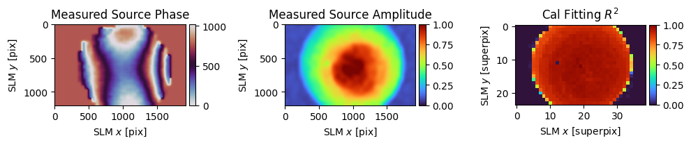
wavefront_cal = fs.process_wavefront_calibration(r2_threshold=.9, smooth=True, plot=True)
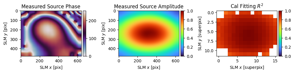
The phase pattern is smooth in the center but the fitting error increases around the panel edges where the illumination amplitude also drops off. The amplitude appears to be spot on (.. no pun intended ..). The real question is – how does the computed flatness map compare to the true phase error?
[10]:
phase_corrected = np.mod(slm.source["phase"]+slm.source["phase_sim"], 2*np.pi)

fig, ax = plt.subplots(1,1)
im = ax.imshow(phase_corrected/(2*np.pi),
               cmap=plt.get_cmap("twilight"),
               interpolation="none")

divider = make_axes_locatable(ax)
cax = divider.append_axes("right", size="5%", pad=0.05)
plt.colorbar(im, cax=cax)
ax.set_title('Wavefront Error');
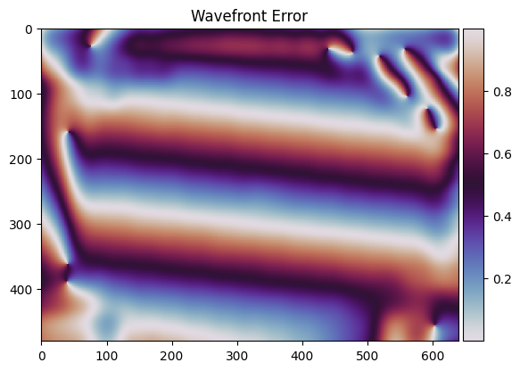
Qualitatively, we’re (primarily) left with a residual blaze where the fitting was good. This makes sense, as any linear phase ramp in the true flatness map is effectively projected out (i.e. corrected) by Fourier calibration which calculates and compensates for the resulting spot translation.
Quantiatively, how good did we do? To find out, let’s try a hologram and compute some spot metrics.
[11]:
# Make the desired hologram: a grid of points on the camera
xlist = np.arange(50, cam.shape[1]-50, 50)
ylist = np.arange(50,cam.shape[0]-50,50)
xgrid, ygrid = np.meshgrid(xlist, ylist)
square = np.vstack((xgrid.ravel(), ygrid.ravel()))
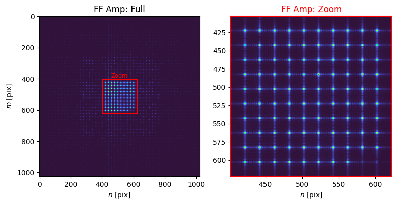
hologram = SpotHologram(shape=slm.shape, spot_vectors=square, basis='ij', cameraslm=fs)
hologram.plot_farfield(hologram.target, title="Target")
C:\Users\Experiment\Documents\GitHub\slmsuite\docs\slmsuite-examples\examples\../../..\slmsuite\holography\algorithms.py:325: UserWarning: algorithms.py: Hologram target shape (480, 640) is not a power of 2; consider using .calculate_padded_shape() to pad to powers of 2 and speed up FFT computation. While some FFT solvers support other prime powers (3, 5, 7, ...), literature suggests that GPU support is best for powers of 2.
  warnings.warn(
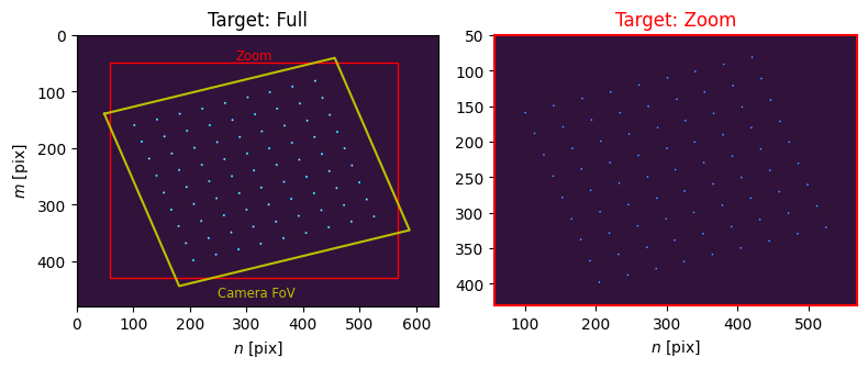
[11]:
[array([ 58, 568], dtype=int64), array([ 50, 431], dtype=int64)]
[12]:
# Callback function: set camera exposure and center spots during first few WGS iterations
def tweaks(holo):
    if holo.iter == 0:
        cam.autoexposure(0.8)
    if holo.iter < 2:
        holo.refine_offset()
    return False

# Run WGS for 50 iterations; fix the far-field phase after 10 iterations
hologram.optimize(
    'WGS-Kim',
    maxiter=50,
    callback = tweaks,
    fix_phase_iteration=10,
    feedback='experimental_spot',
    stat_groups=['computational_spot', 'experimental_spot'])
Reset exposure to 2215.74s; maximum image value = 16384.
Reset exposure to 1107.87s; maximum image value = 16384.
Reset exposure to 553.93s; maximum image value = 16384.
Reset exposure to 276.97s; maximum image value = 16384.
Reset exposure to 138.48s; maximum image value = 16384.
Reset exposure to 69.24s; maximum image value = 16384.
Reset exposure to 34.62s; maximum image value = 11107.
Reset exposure to 25.53s; maximum image value = 8192.
[13]:
plt.imshow(cam.get_image())
plt.colorbar()
[13]:
<matplotlib.colorbar.Colorbar at 0x1bf8aed9250>
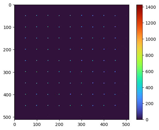
Now let’s visualize the results and calculate a few statistics for comparison.
[14]:
img = cam.get_image()
subimages = analysis.take(img, square, hologram.spot_integration_width_ij)
analysis.take_plot(subimages)
power = analysis.image_normalization(np.array(subimages, dtype=np.float32))
hologram.plot_stats()

# Calculate a few statistics
pos = analysis.image_moment(subimages,moment=(1,0)), analysis.image_moment(subimages,moment=(0,1))
print(r"Spot center = (%1.3f,%1.3f) +/- (%1.3f,%1.3f) px"%(np.mean(pos[0]),np.mean(pos[1]),np.var(pos[0]),np.var(pos[1])))
shape = analysis.image_moment(subimages,moment=(1,1))
print(r"Spot skew = %1.3f +/- %1.3f px"%(np.mean(shape),np.var(shape)**0.5))
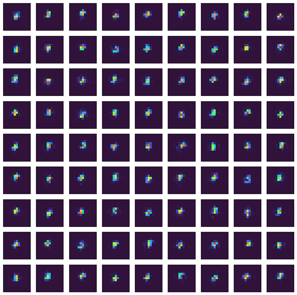
Spot center = (-0.288,-0.570) +/- (0.115,0.214) px
Spot skew = 0.094 +/- 0.300 px
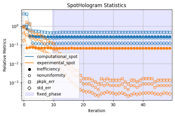
Peak-to-peak power uniformity bottoms out ~\(10^{-3}\). Lets compare the other stats to those generated using: 1) wavefront calibration using phase_steps>1; and 2) perfect wavefront calibration.
[15]:
#1) phase_steps=10
fs.wavefront_calibrate(
    interference_point=(300, 300),
    field_point=(800, 500),
    field_point_units="ij",
    superpixel_size=40,
    phase_steps=10,
    plot=False,
    autoexposure=True);
C:\Users\Experiment\Documents\GitHub\slmsuite\docs\slmsuite-examples\examples\../../..\slmsuite\hardware\cameraslms.py:784: UserWarning: Non-resolvable interference fringe period for the given SLM calibration extent. Either exclude more of the SLM or magnify the field on the camera.
  warnings.warn(
Reset exposure to 81.71s; maximum image value = 30.
Reset exposure to 163.42s; maximum image value = 61.
Reset exposure to 326.85s; maximum image value = 121.
Reset exposure to 653.69s; maximum image value = 242.
Reset exposure to 1307.38s; maximum image value = 484.
Reset exposure to 2614.76s; maximum image value = 968.
Reset exposure to 5229.52s; maximum image value = 1936.
Reset exposure to 10459.04s; maximum image value = 3872.
Reset exposure to 20918.08s; maximum image value = 7745.
The calibration took ~2x longer (and with ~10x more calls to the SLM, which would actually dominate calibration time in an experiment); how did it perform?
[16]:
wavefront_cal = fs.process_wavefront_calibration(r2_threshold=.9, smooth=True, plot=True)
So the result is cleaner, but does better fitting mean better spots? Let’s see…
[17]:
#Redo Fourier cal
fs.fourier_calibrate(
    array_shape=[10, 10],           # Size of the calibration grid (Nx, Ny) [knm]
    array_pitch=[20, 20],           # Pitch of the calibration grid (x, y) [knm]
    plot=False)
[17]:
{'M': array([[ 730.46648446, -237.01203541],
        [ 237.0550149 ,  730.29917439]]),
 'b': array([[258.41746582],
        [252.57378025]]),
 'a': array([[0.],
        [0.]])}
[18]:
hologram = SpotHologram(shape=slm.shape, spot_vectors=square, basis='ij', cameraslm=fs)
hologram.optimize(
    'WGS-Kim',
    maxiter=50,
    callback = tweaks,
    fix_phase_iteration=10,
    feedback='experimental_spot',
    stat_groups=['computational_spot', 'experimental_spot'])
C:\Users\Experiment\Documents\GitHub\slmsuite\docs\slmsuite-examples\examples\../../..\slmsuite\holography\algorithms.py:325: UserWarning: algorithms.py: Hologram target shape (480, 640) is not a power of 2; consider using .calculate_padded_shape() to pad to powers of 2 and speed up FFT computation. While some FFT solvers support other prime powers (3, 5, 7, ...), literature suggests that GPU support is best for powers of 2.
  warnings.warn(
Reset exposure to 2091.81s; maximum image value = 16384.
Reset exposure to 1045.90s; maximum image value = 16384.
Reset exposure to 522.95s; maximum image value = 16384.
Reset exposure to 261.48s; maximum image value = 10827.
Reset exposure to 197.84s; maximum image value = 8192.
[19]:
img = cam.get_image()
subimages = analysis.take(img, square, hologram.spot_integration_width_ij)
power = analysis.image_normalization(np.array(subimages, dtype=np.float32))
# plt.hist(power / np.mean(power)); plt.show()
hologram.plot_stats()

# Calculate a few statistics
pos = analysis.image_moment(subimages,moment=(1,0)), analysis.image_moment(subimages,moment=(0,1))
print(r"Spot center = (%1.3f,%1.3f) +/- (%1.3f,%1.3f) px"%(np.mean(pos[0]),np.mean(pos[1]),np.var(pos[0]),np.var(pos[1])))
shape = analysis.image_moment(subimages,moment=(1,1))
print(r"Spot skew = %1.3f +/- %1.3f px"%(np.mean(shape),np.var(shape)**0.5))
Spot center = (0.005,-0.099) +/- (0.113,0.201) px
Spot skew = -0.067 +/- 0.165 px
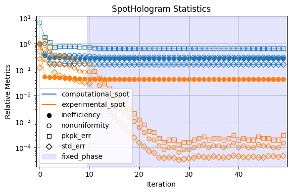
The spot centering, skew, and uniformity are a bit better. How about perfect wavefront calibration?
[20]:
# Perfect calibration: set measured to simulated values
slm.source["phase"] = -slm.source["phase_sim"]
slm.source["amplitude"] = slm.source["amplitude_sim"]
[21]:
#Redo Fourier cal
fs.fourier_calibrate(
    array_shape=[10, 10],           # Size of the calibration grid (Nx, Ny) [knm]
    array_pitch=[20, 20],           # Pitch of the calibration grid (x, y) [knm]
    plot=False)
[21]:
{'M': array([[ 730.60283429, -237.32275852],
        [ 236.99233331,  730.42669537]]),
 'b': array([[255.99969748],
        [255.99601209]]),
 'a': array([[0.],
        [0.]])}
[22]:
hologram = SpotHologram(shape=slm.shape, spot_vectors=square, basis='ij', cameraslm=fs)
hologram.optimize(
    'WGS-Kim',
    maxiter=50,
    callback = tweaks,
    fix_phase_iteration=10,
    feedback='experimental_spot',
    stat_groups=['computational_spot', 'experimental_spot'])
C:\Users\Experiment\Documents\GitHub\slmsuite\docs\slmsuite-examples\examples\../../..\slmsuite\holography\algorithms.py:325: UserWarning: algorithms.py: Hologram target shape (480, 640) is not a power of 2; consider using .calculate_padded_shape() to pad to powers of 2 and speed up FFT computation. While some FFT solvers support other prime powers (3, 5, 7, ...), literature suggests that GPU support is best for powers of 2.
  warnings.warn(
Reset exposure to 158.27s; maximum image value = 8564.
[23]:
img = cam.get_image()
subimages = analysis.take(img, square, hologram.spot_integration_width_ij)
power = analysis.image_normalization(np.array(subimages, dtype=np.float32))
# plt.hist(power / np.mean(power)); plt.show()
hologram.plot_stats()

# Calculate a few statistics
pos = analysis.image_moment(subimages,moment=(1,0)), analysis.image_moment(subimages,moment=(0,1))
print(r"Spot center = (%1.3f,%1.3f) +/- (%1.3f,%1.3f) px"%(np.mean(pos[0]),np.mean(pos[1]),np.var(pos[0]),np.var(pos[1])))
shape = analysis.image_moment(subimages,moment=(1,1))
print(r"Spot skew = %1.3f +/- %1.3f px"%(np.mean(shape),np.var(shape)**0.5))
Spot center = (0.015,-0.088) +/- (0.119,0.184) px
Spot skew = -0.081 +/- 0.168 px
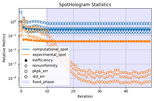
Not much different. So both wavefront calibration routines work well (the single point calibration can also be improved by reducing the lower bound for acceptable values of \(R^2\) fitting quality). As we continue to develop slmsuite, we plan to introduce additional wavefront calibration routines along with better metrics (e.g., Strehl ratio) to study their performance.
Cloning an Experiment into Simulation
Another neat feature of simulation mode is the ability to easily clone an experiment into simulation, thus creating a “digital twin” that can be used to compare observed and ideal performance.
[24]:
from slmsuite.hardware.slms.santec import Santec
from slmsuite.hardware.cameras.alliedvision import AlliedVision
[25]:
slm = Santec(slm_number=1, display_number=2, wav_um=.633, settle_time_s=.3)
cam = AlliedVision(serial="02C5V", verbose=True)
fs = FourierSLM(cam, slm)
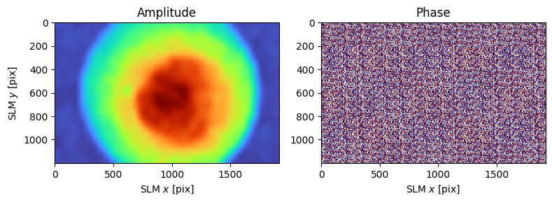
fs.load_wavefront_calibration(plot=True);
Santec slm_number=1 initializing... success
Looking for display_number=2... success
Opening LCOS-SLM,SOC,8001,2018021001... success
vimba initializing... success
Looking for cameras... success
vimba sn 02C5V initializing... success
[26]:
cam.set_exposure(0.01)
fs.fourier_calibrate(
    array_shape=[30, 20],           # Size of the calibration grid (Nx, Ny) [knm]
    array_pitch=[30, 40],           # Pitch of the calibration grid (x, y) [knm]
    plot=True
)
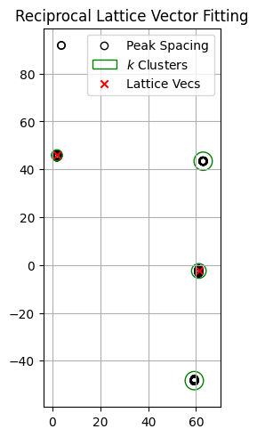
C:\Users\Experiment\Documents\GitHub\slmsuite\docs\slmsuite-examples\examples\../../..\slmsuite\holography\analysis.py:1493: UserWarning: The fitted spot array approaches or exceeds the camera FOV; calibration results may be improperly centered as a result.
  warnings.warn(
[26]:
{'M': array([[-28824.69275653,   1168.11665108],
        [  1180.32581075,  28853.27802505]]),
 'b': array([[560.31675049],
        [550.49759045]]),
 'a': array([[-1.16424394e-20],
        [ 7.45116124e-19]])}
After Fourier and wavefront calibration, we can run a clean hardware-based experiment.
[27]:
xlist = np.linspace(400, 600, 10)
ylist = np.linspace(200, 400, 10)
xgrid, ygrid = np.meshgrid(xlist, ylist)
square = np.vstack((xgrid.ravel(), ygrid.ravel()))
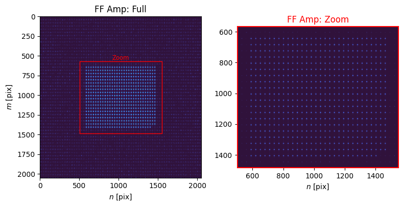
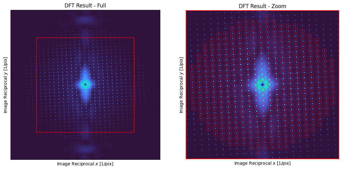
hologram = SpotHologram(shape=slm.shape, spot_vectors=square, basis='ij', cameraslm=fs)
hologram.plot_farfield(hologram.target, title="Target")
C:\Users\Experiment\Documents\GitHub\slmsuite\docs\slmsuite-examples\examples\../../..\slmsuite\holography\algorithms.py:325: UserWarning: algorithms.py: Hologram target shape (1200, 1920) is not a power of 2; consider using .calculate_padded_shape() to pad to powers of 2 and speed up FFT computation. While some FFT solvers support other prime powers (3, 5, 7, ...), literature suggests that GPU support is best for powers of 2.
  warnings.warn(
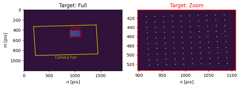
[27]:
[array([ 897, 1109], dtype=int64), array([402, 534], dtype=int64)]
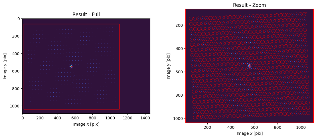
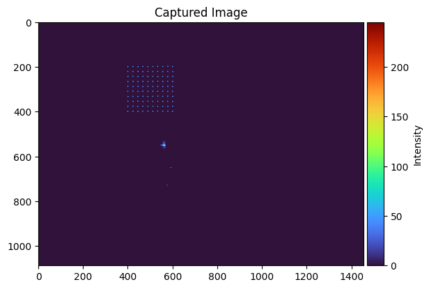
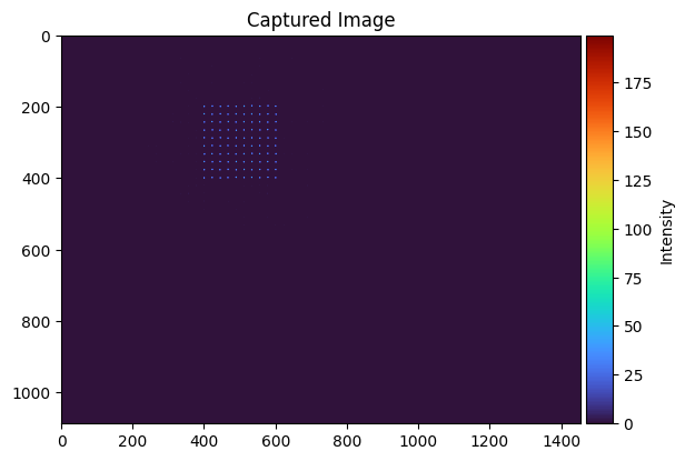
[28]:
cam.set_exposure(0.004)

hologram.optimize(
    'WGS-Kim',
    maxiter=30,
    fix_phase_iteration=10,
    feedback='experimental_spot',
    stat_groups=['computational_spot', 'experimental_spot'])

cam.get_image(plot=True)
ax = hologram.plot_stats()
ax.set_title('Experimental Convergence')
C:\Users\Experiment\Documents\GitHub\slmsuite\docs\slmsuite-examples\examples\../../..\slmsuite\holography\algorithms.py:1327: RuntimeWarning: divide by zero encountered in divide
  feedback_pwr *= 1 / feedback_pwr_sum
C:\Users\Experiment\Documents\GitHub\slmsuite\docs\slmsuite-examples\examples\../../..\slmsuite\holography\algorithms.py:1327: RuntimeWarning: invalid value encountered in multiply
  feedback_pwr *= 1 / feedback_pwr_sum
C:\Users\Experiment\Documents\GitHub\slmsuite\docs\slmsuite-examples\examples\../../..\slmsuite\holography\algorithms.py:1328: RuntimeWarning: divide by zero encountered in divide
  feedback_amp *= 1 / xp.sqrt(feedback_pwr_sum)
C:\Users\Experiment\Documents\GitHub\slmsuite\docs\slmsuite-examples\examples\../../..\slmsuite\holography\algorithms.py:1328: RuntimeWarning: invalid value encountered in multiply
  feedback_amp *= 1 / xp.sqrt(feedback_pwr_sum)
[28]:
Text(0.5, 1.0, 'Experimental Convergence')
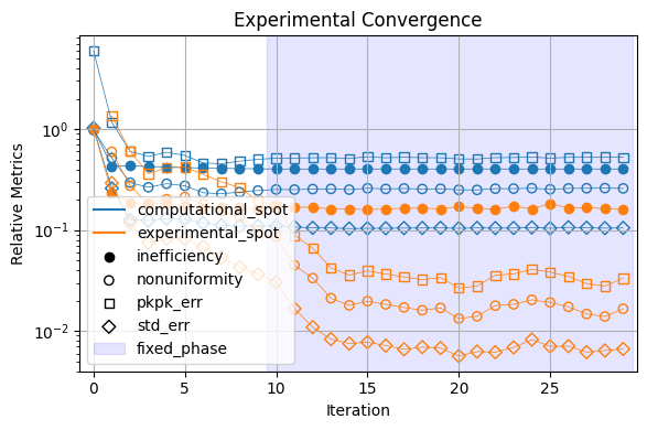
We can easily compare the results to ideal performance using slmsuite’s simulation features. The simulate method of FourierSLM creates simulated replicas of the camera and SLM and orients them according to the measured Fourier calibration.
[29]:
fs_sim = fs.simulate()
Padded SLM k-space shape set to (4096,4096) to achieve required imaging resolution.
[31]:
hologram_sim = SpotHologram(shape=fs_sim.slm.shape, spot_vectors=square, basis='ij', cameraslm=fs_sim)
fs_sim.cam.set_exposure(800)

hologram_sim.optimize(
    'WGS-Kim',
    maxiter=30,
    fix_phase_iteration=10,
    feedback='experimental_spot',
    stat_groups=['computational_spot', 'experimental_spot'])

fs_sim.cam.get_image(plot=True)
ax = hologram_sim.plot_stats()
ax.set_title('Simulated Convergence')
[31]:
Text(0.5, 1.0, 'Simulated Convergence')
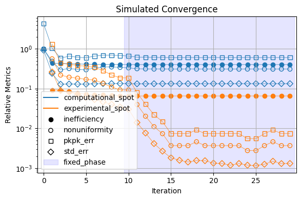
We can now see that the experimental convergence is slightly worse than the camera-bit-depth-limited (simulated) performance. We can now use slmsuite to hunt down the source of the discrepancy.