Multiplane Holography

The previous slmsuite examples have examined holography powered by discrete Fourier transforms (DFTs) and by “compressed” Zernike kernels. We now examine a sort of meta holography which “bakes” many simple objectives into a single hologram. These objectives can span planes of focus (DFTs or spots at different \(z\) positions), planes of color (DFT grids or kernels scaled for different wavelengths), planes of basis (combining DTF and kernel objectives into the same hologram), or more!

Initialization

To start, we initialize our system:

# Try to load physical hardware.
try:
    from slmsuite.hardware.slms.texasinstruments import PLM
    from slmsuite.hardware.cameras.flir import FLIR

    # Load the hardware.
    slm = PLM('p67', 1, wav_um=0.488, settle_time_s=0.05, configure_usb=True); print()
    cam = FLIR(serial="22562470", pitch_um=2.74, bitdepth=12)

    # For this camera, we also want to crop the WOI to the center 1024x1024 area.
    h_max, w_max = cam.default_shape
    d_im = 1920
    cam.set_woi(((w_max - d_im) // 2, d_im, (h_max - d_im) // 2, d_im))

    # Load the composite CameraSLM.
    fs = FourierSLM(cam, slm)
    fs.load_calibration("wavefront_superpixel");
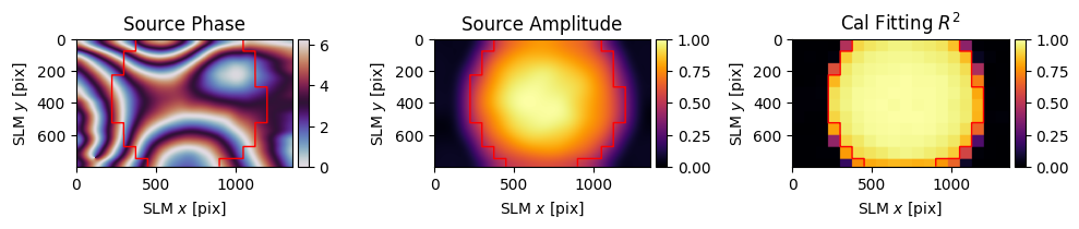
    fs.wavefront_calibration_superpixel_process(plot=True, r2_threshold=.8)
# Fallback to virtual hardware.
except Exception as e:
    print(f"Loading physical hardware failed; loading virtual hardware. Error:\n{str(e)}")
    from slmsuite.hardware.slms.simulated import SimulatedSLM
    from slmsuite.hardware.cameras.simulated import SimulatedCamera

    # Make the SLM and camera.
    slm = SimulatedSLM((1600, 1200), pitch_um=(8,8))
    # Program the simulated and calibrated sources to be flat phase.
    slm.set_source_analytic(sim=True)
    slm.set_source_analytic()

    cam = SimulatedCamera(slm, (1440, 1100), pitch_um=(4,4), gain=200)

    # Tie the camera and SLM together with an analytic calibration.
    fs = FourierSLM(cam, slm)
    M, b = fs.fourier_calibration_build(
        f_eff=80000.,                              # f_eff of 80000 wavelengths or 80 mm with the default 1 um wavelength
        theta=5 * np.pi / 180,
    )
    cam.set_affine(M, b)
    fs.fourier_calibrate_analytic(M, b)

PLM using GPU (cupy) backend
DLPC900 connected: firmware {'app_version': 95, 'api_version': 72, 'sw_patch': 111, 'sw_minor': 108, 'sw_major': 111}
DLPC900 pre-configured (video mode, display detected)
Initializing pyglet... success
Searching for window with display_number=1... success
Creating window... Window creation successful
DLPC900 source locked, switching to video-pattern mode...
DLPC900 configured successfully - pattern sequence running

PySpin initializing... Looking for cameras... PySpin sn '22562470' initializing... PixelFormat set to Mono16 (12-bit)... Frame rate set to 11.8 Hz... Successfully initialized FLIR cam 22562470.

C:\Users\holodyne\Documents\GitHub\slmsuite\slmsuite\hardware\cameraslms.py:3720: UserWarning: remove_background is enabled and a noise floor was detected; removing this background (0.07164789736270905% of the average normalization).
  warnings.warn(

exposure_base = 0.1
cam.set_exposure(exposure_base)
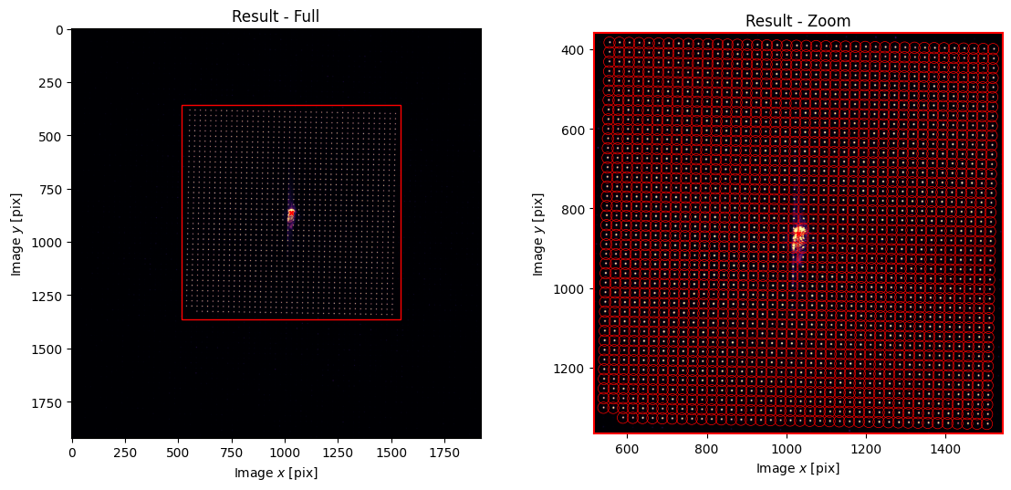
fs.fourier_calibrate(40, 20, plot=True);

C:\Users\holodyne\Documents\GitHub\slmsuite\slmsuite\holography\toolbox\__init__.py:258: UserWarning: CameraSLM must be passed as slm for conversion 'kxy' to 'ij'
  warnings.warn(

We make a function to help with building our banner image.

# Helper function for setting up banner sizes and MRAF on images.
path = os.path.join(os.getcwd(), '../../slmsuite/docs/source/static/slmsuite-small.png')

from slmsuite.holography.analysis.files import _load_image
from slmsuite.holography.toolbox.phase import lens

h, w = banner_shape = (640, 1280)
x, y = banner_shift = (0, -215)

y0, x0 = np.array(cam.shape) / 2

x += x0
y += y0

i0,i1,i2,i3 = (int(y-h/2), int(y+h/2), int(x-w/2), int(x+w/2))

def load_img(path):
    target_ij = _load_image(path, cam.shape, shift=(-225, -170))

    # Fill with nan for MRAF outside the bounds of the banner.
    p = 5

    target_ij[:(i0-p), :] = np.nan
    target_ij[(i1+p):, :] = np.nan
    target_ij[:, :(i2-p)] = np.nan
    target_ij[:, (i3+p):] = np.nan

    return target_ij

Planes of Focus

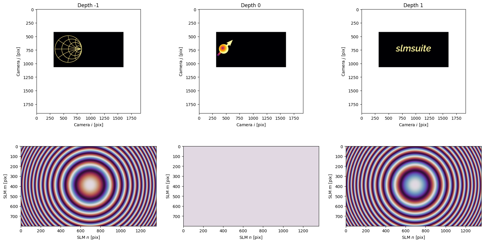
Optimizing a hologram at a detuned \(z\) position is as simple as adding a given propogation_kernel to the DFT which maps the nearfield of the SLM to the farfield. Instead of being located at exactly the depth of focus of the system, the DFT grid will instead follow the detuned focus (and aberration) of the propogation_kernel. We can make a series of holograms (comprising the three parts of our logo) at different depths. Here, the depth is determined by the lens(f) phase function, which adds a lens with focal length \(f\) to our system at the plane of the SLM. The case of \(f=\infty\) corresponds to no lens.

from slmsuite.holography.algorithms import FeedbackHologram

f_eff_target = 1e7
targets = []
kernels = []
holograms = []
weights = []

# Gather three objectives for a fancy slmsuite logo.
for sym, f_eff in zip(["smith", "spin", "text"], [-f_eff_target, np.inf, f_eff_target]):
    target_ij = load_img(os.path.join(os.getcwd(), f'../../slmsuite/docs/source/static/slmsuite-small-{sym}.png'))
    kernel = lens(slm, f_eff)

    targets.append(target_ij)
    kernels.append(kernel)
    holograms.append(
        FeedbackHologram(
            (2048, 2048),
            target_ij,
            null_region_radius_frac=.5,                 # Helper function for MRAF.
            cameraslm=fs,
            propagation_kernel=lens(slm, f_eff)         # We're setting different planes of focus here with an appropriate lens().
        )
    )
    weights.append(np.sqrt(np.nansum(np.square(target_ij.astype(float)))))

This is what we loaded: three parts of a now-3D image with the encoded desired depths.

fig, axs = plt.subplots(2, 3, figsize=(20,10)); axs=axs.ravel()

for i, target, kernel in zip(range(3), targets, kernels):
    cam.plot(target, title=f"Depth {i-1}", ax=axs[i], cbar=False)
    slm.plot(kernel, title="", ax=axs[3+i], cbar=False)

We can now make a meta-hologram out of these FeedbackHologram objectives. The weights factors encodes the relative weight of each objective, as the intensity of the image is lost when each is normalized upon FeedbackHologram initialization.

from slmsuite.holography.algorithms import MultiplaneHologram

mh = MultiplaneHologram(holograms=holograms, weights=weights)

Next, we optimize. Here, we initialize with a quadratic phase guess and apply MRAF to reduce speckle.

mh.reset_phase(random_phase=0, quadratic_phase=2)
mh.optimize(method="GS", maxiter=5, mraf_factor=1)
mh.optimize(method="WGS-Leonardo", maxiter=20, mraf_factor=.5, feedback="computational")

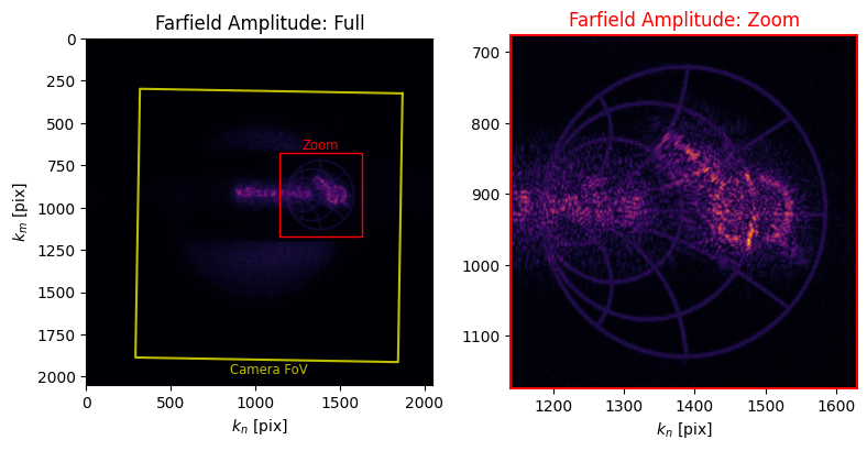
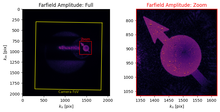
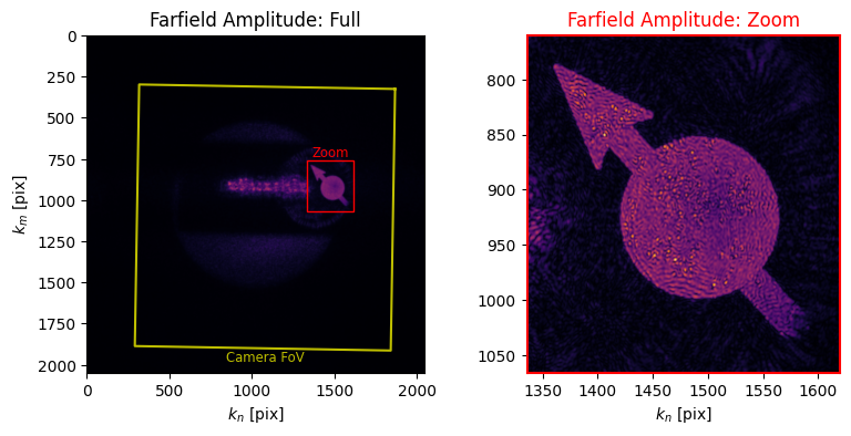
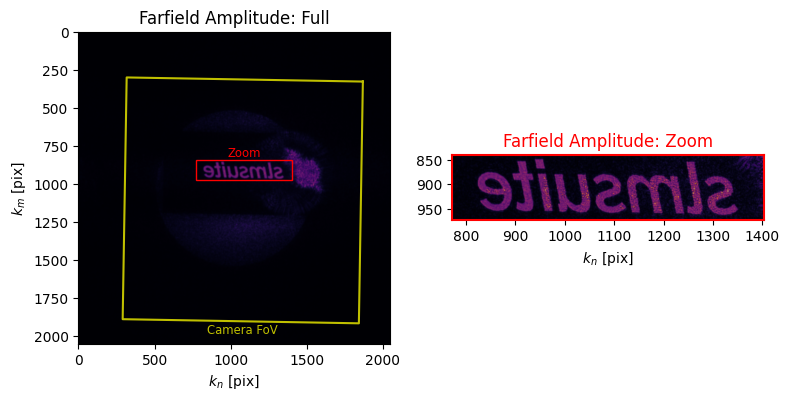
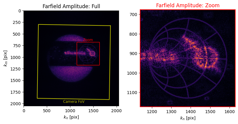
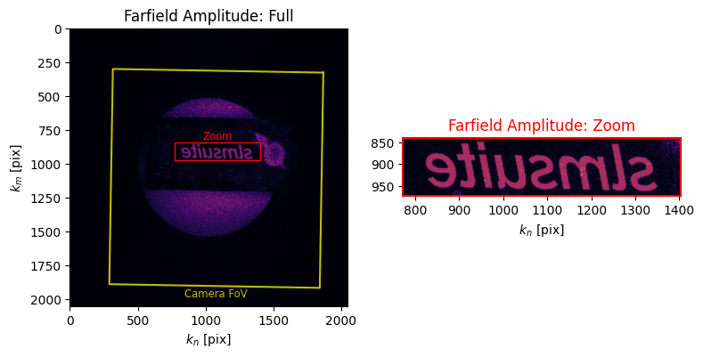
We can take a first look at our result by looking at the computational farfield. This calls .plot_farfield() for each of the child holograms, and each farfield is examined with the desired propagation kernel applied. It is this farfield which is optimized against.

mh.plot_farfield()

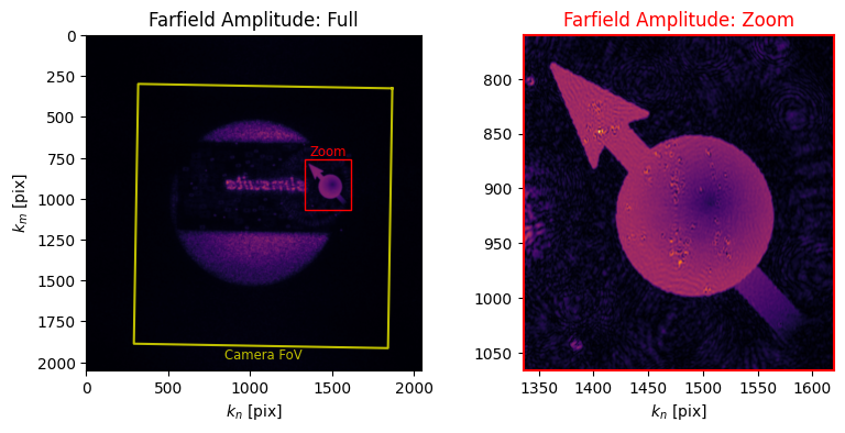
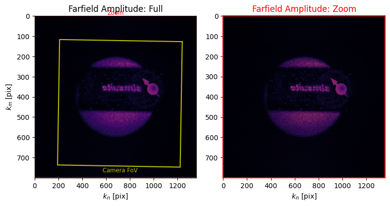
But we can do more than this. Image feedback works the same way for multiplane holograms, except this time the propagation_kernel is used to focus the spot for each experimental feedback image. This takes a bit longer because we settle three times and capture three images (one for each plane) during each iteration.

mh.optimize(method="WGS-tanh", maxiter=10, mraf_factor=.5, feedback_factor=.5, feedback_exponent=10, feedback="experimental")

mh.plot_farfield()

Now let’s take a look at the final result.

import tqdm.auto as tqdm

osc = (1/f_eff_target) * np.sin(np.linspace(0, 2*np.pi, 25))

imgs = []

for f in tqdm.tqdm(np.reciprocal(osc)):
    slm.set_phase(mh.get_phase() + lens(slm, f))
    cam.flush()
    img_ij = cam.get_image()

    banner = img_ij[i0:i1, i2:i3]
    imgs.append(banner)

C:\Users\holodyne\AppData\Local\Temp\ipykernel_38992\3082363685.py:7: RuntimeWarning: divide by zero encountered in reciprocal
  for f in tqdm.tqdm(np.reciprocal(osc)):

from slmsuite.holography.analysis.files import save_image

save_image("ex-mutiplane.gif", imgs, cmap="Blues", normalize=False, loop=0)
save_image("ex-mutiplane-dark.gif", imgs, cmap="inferno", normalize=False, loop=0)

Planes of Basis

Alongside meta objectives consisting of many DFT holograms at different planes of focus, we can combine DFT- and kernel/spot- based objectives in the same hologram. This image is used for the slmsuite banner image on GitHub. We first again load our image, this time in a single plane because in the end we will want to have a static image instead of a .gif.

from slmsuite.holography.algorithms import FeedbackHologram

holograms = []
weights = []

# Load the image.
target_ij = load_img(os.path.join(os.getcwd(), f'../../slmsuite/docs/source/static/slmsuite-small.png'))

holograms.append(
    FeedbackHologram(
        (2048, 2048),
        target_ij,
        null_region_radius_frac=.5,
        cameraslm=fs
    )
)

For the spots, we want to make two Zernike pyramids. One is the usual that we made in a previous example. The other makes use of a secret less-documented Zernike index -1. This is nonsensical as an ANSI Zernike index, but in slmsuite it is the keyword for a \(LG_{pl} = LG_{01}\) polynomial or vortex waveplate which produces a bottle beam in the farfield. In the future, we might support more special keywords in the negative integers.

from slmsuite.holography.algorithms import CompressedSpotHologram
from slmsuite.holography.toolbox import convert_vector
from slmsuite.holography.toolbox.phase import zernike_convert_index

# Make two pyramids of order 7 in the camera basis.
N = 28
i = np.arange(N)
nl = zernike_convert_index(i, from_index="ansi", to_index="radial")
p = 27
x = cam.shape[1]/2 + 400
y = cam.shape[0]/2 + banner_shift[1]

vectors_ij = np.hstack((
    np.vstack((x + p * nl[:, 1], y - p * (1 + nl[:, 0] * np.sqrt(3)))),
    np.vstack((x + p * nl[:, 1], y + p * (1 + nl[:, 0] * np.sqrt(3))))
))

# Then convert to the Zernike basis and add a pertubation.
vectors_zernike_xy = convert_vector(
    vectors_ij,
    from_units="ij",
    to_units="zernike",
    hardware=fs
)

vectors_zernike = np.zeros((N,2*N))
vectors_zernike[2, :] = vectors_zernike_xy[0]
vectors_zernike[1, :] = vectors_zernike_xy[1]

perturbation = np.diag(np.ones(N))
perturbation = np.hstack((perturbation, perturbation))

vectors_zernike_pyramid = vectors_zernike + 10*perturbation

# Give the upper pyramid a LG03 term.
vectors_zernike_final = np.vstack((vectors_zernike_pyramid, np.zeros(2*N)))
vectors_zernike_final[-1, :N] = 3 # LG03
basis = np.hstack((i, [-1]))

holograms.append(
    CompressedSpotHologram(
        spot_vectors=vectors_zernike_final,
        basis=basis,
        cameraslm=fs
    )
)

C:\Users\holodyne\Documents\GitHub\slmsuite\slmsuite\holography\algorithms\_spots.py:360: UserWarning: Found ANSI index '0' (Zernike piston) in the zernike_basis; this is not necessary as spot phase is controlled externally.
  warnings.warn(

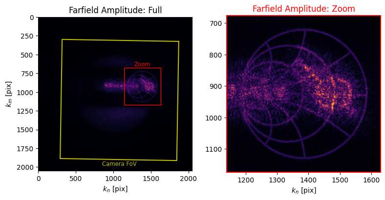
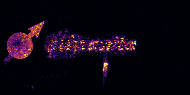
Finally, we make and optimize the meta-hologram. Here, the weights are less balanced than the previous example, but that’s expected because the Zernike pyramids need comparatively smaller power.

from slmsuite.holography.algorithms import MultiplaneHologram

mh = MultiplaneHologram(holograms=holograms, weights=[1, .5])

mh.reset_phase(random_phase=0, quadratic_phase=2)
mh.optimize(method="WGS-Leonardo", maxiter=10, mraf_factor=1, feedback_exponent=.8, feedback="computational")

mh.plot_farfield()

mh.optimize(method="WGS-tanh", maxiter=40, mraf_factor=.5, feedback_factor=.5, feedback_exponent=5, feedback="experimental")

C:\Users\holodyne\Documents\GitHub\slmsuite\slmsuite\holography\algorithms\_spots.py:942: UserWarning: CompressedSpotHologram feedback 'experimental' is interpreted as 'experimental_spot'
  warnings.warn("CompressedSpotHologram feedback 'experimental' is interpreted as 'experimental_spot'")

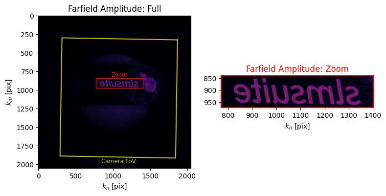
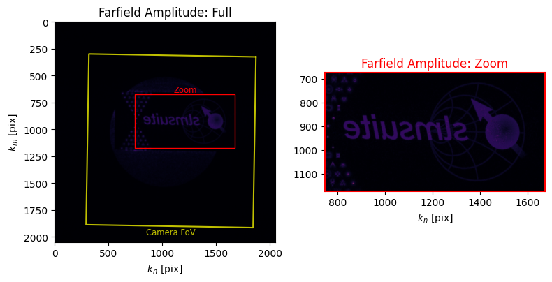
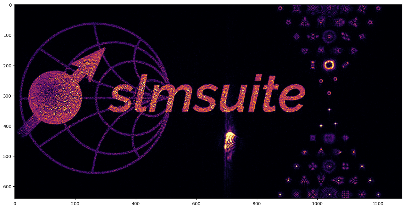
Now let’s collect the banner!

slm.set_phase(mh.get_phase())
img_ij = cam.get_image()

banner = img_ij[i0:i1, i2:i3]

plt.figure(figsize=(16,8))
plt.imshow(banner)
plt.show()

save_image("slmsuite-banner.png", banner, cmap=True, border=127)

Planes of Both

As a final example hologram, let’s combine the two previous cases. We want to make the 3D slmsuite logo moving through a starfield of bottle beams.

from slmsuite.holography.algorithms import FeedbackHologram

f_eff_target = 1e7
targets = []
kernels = []
holograms = []
weights = []

# Gather three objectives for a fancy slmsuite logo.
for sym, f_eff in zip(["smith", "spin", "text"], [-f_eff_target, np.inf, f_eff_target]):
    target_ij = load_img(os.path.join(os.getcwd(), f'../../slmsuite/docs/source/static/slmsuite-small-{sym}.png'))
    kernel = lens(slm, f_eff)

    targets.append(target_ij)
    kernels.append(kernel)
    holograms.append(
        FeedbackHologram(
            (2048, 2048),
            target_ij,
            null_region_radius_frac=.5,                 # Helper function for MRAF.
            cameraslm=fs,
            propagation_kernel=lens(slm, f_eff)         # We're setting different planes of focus here with an appropriate lens().
        )
    )

    weights.append(np.sqrt(np.nansum(np.square(target_ij.astype(float)))))

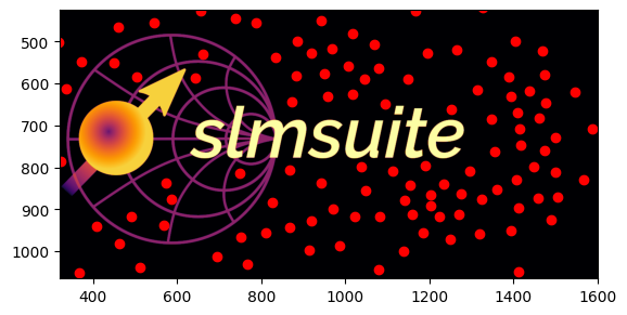
Now we move onto the bottle beams. We use the same ANSI index -1 as before to add a vortex waveplate term to the Zernike basis. For clarity, we also tell the spots to avoid the DFT holograms via blurring and each other via lloyds_algorithm().

from slmsuite.holography.algorithms import CompressedSpotHologram
import cv2

# Make the starfield
# Points
N_spots = 200

spots_ij = np.vstack((
    np.random.randint(i2, i3, size=N_spots),
    np.random.randint(i0, i1, size=N_spots)
))

from slmsuite.holography.toolbox import lloyds_algorithm
from slmsuite.holography.analysis import _generate_grid

spots_ij = lloyds_algorithm(
    _generate_grid(cam.shape[1], cam.shape[0]),
    spots_ij,
    iterations=2
).astype(int)

# Remove points which are close of the logo.
target_ij = load_img(
    os.path.join(os.getcwd(), f'../../slmsuite/docs/source/static/slmsuite-small.png')
)

target_ij_blur = cv2.GaussianBlur(target_ij.astype(np.uint8), (61,61), 0)

nooverlap = np.logical_and(
    target_ij_blur[spots_ij[1], spots_ij[0]] == 0,
    np.logical_not(np.isnan(target_ij[spots_ij[1], spots_ij[0]]))
)
spots_ij = spots_ij[:, nooverlap]
N_spots = spots_ij.shape[1]

plt.imshow(target_ij)
plt.scatter(spots_ij[0], spots_ij[1], c="r")
plt.ylim(i1, i0)
plt.xlim(i2, i3)
plt.show()

# Convert to kxy units so we can add on depth in units of focal power.
spots_kxy = convert_vector(
    spots_ij,
    from_units="ij",
    to_units="kxy",
    hardware=fs
)

spots_kxyz = np.vstack((
    spots_kxy,
    2 * (np.random.rand(N_spots) - .5) / f_eff_target
))

# Finally, convert to zernike.
spots_zernike = convert_vector(
    spots_kxyz,
    from_units="kxy",
    to_units="zernike",
    hardware=fs
)

# Turn every spot into a bottle beam.
basis = [
    2,      # x
    1,      # y
    4,      # z
    -1      # LG10 - vortex waveplate
]

spots_zernike = np.vstack((
    spots_zernike,
    2 * np.ones((1, N_spots))   # LG20 on every spot, for fun.
))

# Make the spot hologram.
holograms.append(
    CompressedSpotHologram(
        spot_vectors=spots_zernike,
        basis=basis,
        cameraslm=fs
    )
)
weights.append(1000)

C:\Users\holodyne\AppData\Local\Temp\ipykernel_38992\2314959749.py:27: RuntimeWarning: invalid value encountered in cast
  target_ij_blur = cv2.GaussianBlur(target_ij.astype(np.uint8), (61,61), 0)

Making the hologram, optimizing, and monitoring the result is as simple as before:

from slmsuite.holography.algorithms import MultiplaneHologram

mh = MultiplaneHologram(holograms=holograms, weights=weights)

mh.reset_phase(random_phase=0, quadratic_phase=2)
mh.optimize(method="GS", maxiter=5, mraf_factor=1)
mh.optimize(method="WGS-Leonardo", maxiter=20, mraf_factor=1, feedback="computational")

mh.plot_farfield()

mh.optimize(method="WGS-tanh", maxiter=20, mraf_factor=.5, feedback_factor=.5, feedback_exponent=5, feedback="experimental")

C:\Users\holodyne\Documents\GitHub\slmsuite\slmsuite\holography\algorithms\_spots.py:942: UserWarning: CompressedSpotHologram feedback 'experimental' is interpreted as 'experimental_spot'
  warnings.warn("CompressedSpotHologram feedback 'experimental' is interpreted as 'experimental_spot'")

We again collect the spots, oscillating in \(z\).

import tqdm.auto as tqdm

osc = (1/f_eff_target) * np.sin(np.linspace(0, 2*np.pi, 25))

imgs = []

for f in tqdm.tqdm(np.reciprocal(osc)):
    slm.set_phase(mh.get_phase() + lens(slm, f))
    cam.flush()
    img_ij = cam.get_image()

    banner = img_ij[i0:i1, i2:i3]
    imgs.append(banner)

C:\Users\holodyne\AppData\Local\Temp\ipykernel_38992\3082363685.py:7: RuntimeWarning: divide by zero encountered in reciprocal
  for f in tqdm.tqdm(np.reciprocal(osc)):

from slmsuite.holography.analysis.files import save_image

# The .gifs are a bit large at raw resolution for GitHub unfortunately, so we downscale by 2x
N = 2
imgs = np.array(imgs)
imgs2 = 0

for x in range(N):
    for y in range(N):
        imgs2 += imgs[:, x::N, y::N] // (N * N)

save_image("ex-slmsuite-3d.gif", imgs2, cmap="Blues", border=127, normalize=False, loop=0)
save_image("ex-slmsuite-3d-dark.gif", imgs2, cmap="inferno", border=127, normalize=False, loop=0)

Looking at this hologram directly by eye reveals all the depth cues that are lost by image capture on a camera. These depth cues are important for AR/VR applications.

Afterword

Altogether, MultiplaneHologram enhances the versatility of holography with slmsuite Wherever the user is interested in the state of the farfield, at whichever focus or color, the user can wrest control in the form of DFT grids or spots in aberration-space.

We look forward to seeing the novel combinations of objectives you will create!

slm.close()
cam.close()