Multipoint Calibration

Anisoplanatism, spatially-varying aberration across the field of view, is not entirely compensated for by global wavefront calibration. In general, setups with higher NA or setups that image into materials will suffer from higher anisoplanatic aberration.

We want to build upon the wavefront calibration explored in a previous example by calibrating at many points across the field of view simultaneously. slmsuite is equipped with two methods for this:

• A version of the superpixel-based calibration explored before, which interferes many calibration points simultaneously,

• Zernike-based wavefront calibration, where aberration is iteratively subtracted from a Zernike spot array.

Initialization

To start, we initialize our system:

# Try to load physical hardware.
try:
    from slmsuite.hardware.slms.texasinstruments import PLM
    from slmsuite.hardware.cameras.flir import FLIR

    # Load the hardware.
    slm = PLM('p67', 1, wav_um=0.488, settle_time_s=0.05, configure_usb=True); print()
    cam = FLIR(serial="22562470", pitch_um=2.74, bitdepth=12)

    # For this camera, we also want to crop the WOI to the center 1024x1024 area.
    h_max, w_max = cam.default_shape
    cam.set_woi(((w_max - 1024) // 2, 1024, (h_max - 1024) // 2, 1024))

    # Load the composite CameraSLM.
    fs = FourierSLM(cam, slm)
# Fallback to virtual hardware.
except Exception as e:
    print(f"Loading physical hardware failed; loading virtual hardware. Error:\n{str(e)}")
    from slmsuite.hardware.slms.simulated import SimulatedSLM
    from slmsuite.hardware.cameras.simulated import SimulatedCamera

    # Make the SLM and camera.
    slm = SimulatedSLM((1600, 1200), pitch_um=(8,8))
    # Program the simulated and calibrated sources to be flat phase.
    slm.set_source_analytic(sim=True)
    slm.set_source_analytic()

    cam = SimulatedCamera(slm, (1440, 1100), pitch_um=(4,4), gain=200)

    # Tie the camera and SLM together with an analytic calibration.
    fs = FourierSLM(cam, slm)
    M, b = fs.fourier_calibration_build(
        f_eff=80000.,                              # f_eff of 80000 wavelengths or 80 mm with the default 1 um wavelength
        theta=5 * np.pi / 180,
    )
    cam.set_affine(M, b)
    fs.fourier_calibrate_analytic(M, b)

PLM using GPU (cupy) backend
DLPC900 connected: firmware {'app_version': 95, 'api_version': 72, 'sw_patch': 111, 'sw_minor': 108, 'sw_major': 111}
DLPC900 pre-configured (video mode, display detected)
Initializing pyglet... success
Searching for window with display_number=1... success
Creating window... Window creation successful
DLPC900 source locked, switching to video-pattern mode...
DLPC900 configured successfully - pattern sequence running

PySpin initializing... Looking for cameras... PySpin sn '22562470' initializing... PixelFormat set to Mono16 (12-bit)... Frame rate set to 33.7 Hz... Successfully initialized FLIR cam 22562470.

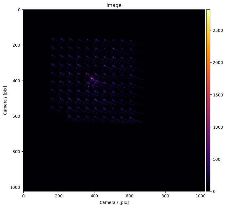
We’ve put in a piece of warped plastic (tupperware) into our setup to induce additional anisoplanatic aberration. If we project the grid used for Fourier calibration, we can see that it’s going to be difficult to get a good fit.

cam.set_exposure(.01)
fs.fourier_grid_project(10, 40)
cam.plot()

C:\Users\holodyne\Documents\GitHub\slmsuite\slmsuite\holography\toolbox\__init__.py:258: UserWarning: CameraSLM must be passed as slm for conversion 'kxy' to 'ij'
  warnings.warn(

<Axes: title={'center': 'Image'}, xlabel='Camera $i$ [pix]', ylabel='Camera $j$ [pix]'>

Thus, we start out by removing the lowest order aberration term: the focusing term \(Z_4\). We use the built-in cam.autofocus() method which accepts general function handles to set_z the position of a stage or otherwise. cam.autofocus() also accepts an SLM as set_z, where the unit of the \(z\) coordinate is in Zernike units: radians times \(Z_4\).

cam.autofocus(
    set_z=slm,
    plot=True,
    range_z=np.linspace(-10, 10, 21, endpoint=True)
)

-3.850716698143393

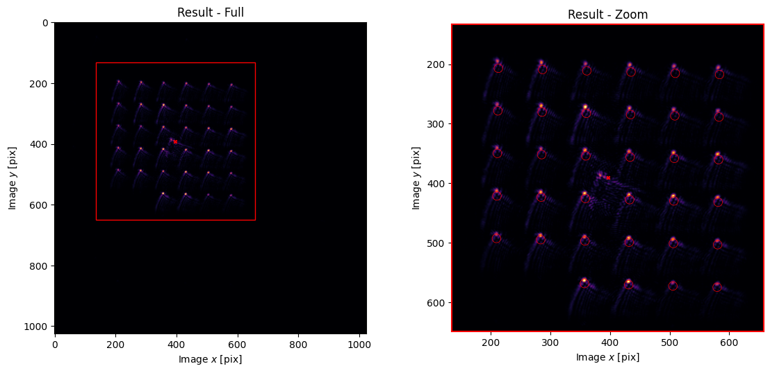
With cam.autofocus() to help us, we are able to get tight enough spots to lock onto the array.

fs.fourier_calibrate(6, 60, plot=True);

Multipoint Calibration Grid

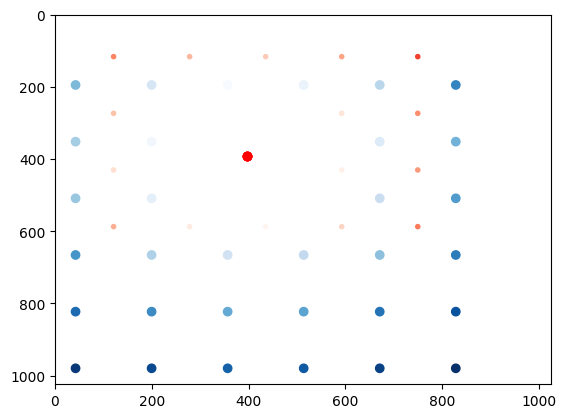
When calibrating at many points, we must be considerate of effects which are not present in single-point calibration. Specifically, each calibration point has a -1th order mirror in addition to the target 1st order location. These -1th orders act as noise for the other points. However, careful choice of how the grid of calibration points is aligned can lead to these mirror images avoiding sensitive regions. This is handled automatically by .wavefront_calibration_points(). In the below plot, the red spots are mirror images of the blue spots, with the intensity corresponding to the spot index.

points_ij = fs.wavefront_calibration_points(pitch=180, avoid_mirrors=True, plot=True);

Multipoint Superpixel Wavefront Calibration

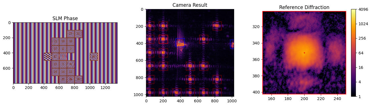
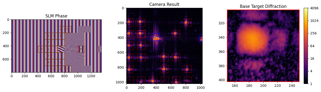
To start, we explore an extension to superpixel-based calibration where we calibrate many points simultaneously. Using the calibration_points=None, the field of view is densely packed with interference regions which are of appropriate size and of sufficient separation for the given superpixel_size.

movie = fs.wavefront_calibrate_superpixel(
    calibration_points=points_ij,
    field_point=(.25, 0),
    field_point_units="freq",
    superpixel_size=100,
    test_index=2,                       # Testing mode
    phase_steps=10,
    plot=3                              # Special mode to generate a phase .gif
)

from slmsuite.holography.analysis.files import save_image

save_image("wavefront-simutaneous.gif", movie, loop=0)

We use markdown to display the .gif we just made:

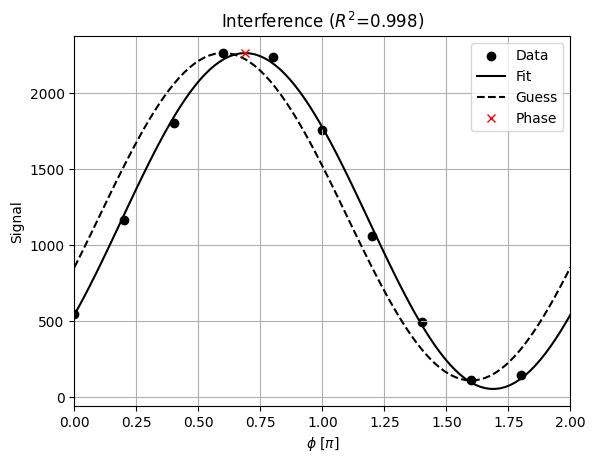
To summarize what is happening: we’re doing many interference measurements at once. For each interference measurement, there is a superpixel pair, one of which has a shifting phase (as seen in the .gif).

Some of the calibration points are not measured during this frame because there is a conflict with another pair. There’s a complex scheduling algorithm running in the background to make sure all pairs of reference and target superpixels are measured despite these conflicts.

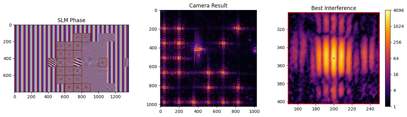
Next, we perform the full calibration:

fs.wavefront_calibrate_superpixel(
    calibration_points=points_ij,
    field_point=(.25, 0),
    field_point_units="freq",
    superpixel_size=100,
    phase_steps=6,
);

C:\Users\holodyne\Documents\GitHub\slmsuite\slmsuite\hardware\cameraslms.py:2773: OptimizeWarning: Covariance of the parameters could not be estimated
  popt, _ = optimize.curve_fit(cos, phases, intensities, p0=guess)

C:\Users\holodyne\Documents\GitHub\slmsuite\slmsuite\holography\analysis\__init__.py:1016: OptimizeWarning: Covariance of the parameters could not be estimated
  popt, pcov = curve_fit(function, grid_ravel_, img, ftol=1e-5, p0=p0,)

The slightly longer runtime compared with single point calibration is due to scheduling against conflicting superpositions positions, alongside overhead of fitting many results every iteration.

fs.save_calibration("wavefront_superpixel")

'c:\\Users\\holodyne\\Documents\\GitHub\\slmsuite-examples\\examples\\22562470-p67-wavefront_superpixel-calibration_00012.h5'

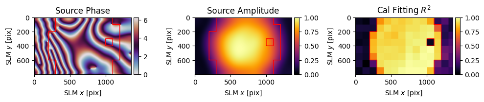
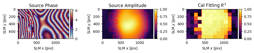
Now let’s take a look at the results of the calibrations at the corners of the field of view.

# Make a grid of spots.
xlist = np.arange(50, min(fs.cam.shape)-50, 100)                      # Get the coordinates for one edge
xgrid, ygrid = np.meshgrid(xlist, xlist)
square = np.vstack((xgrid.ravel(), ygrid.ravel()))                  # Make an array of points in a grid

from slmsuite.holography.algorithms import SpotHologram
hologram = SpotHologram(shape=(2048, 2048), spot_vectors=square, basis='ij', cameraslm=fs)
hologram.optimize(iterations=10, plot=True)

# Find the four corner indices to plot.
points = fs.calibrations["wavefront_superpixel"]["calibration_points"]
corner_indices = []
for x in [-1, 1]:
    for y in [-1, 1]:
        max_corner = x * points[0] + y * points[1]
        corner_indices.append(np.argmax(max_corner))

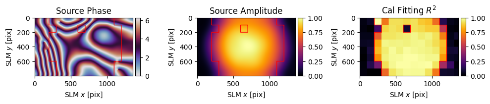
# For each corner index, plot the correction wavefront and the resulting hologram aberration.
for i in corner_indices:
    dat = fs.wavefront_calibration_superpixel_process(index=i, r2_threshold=.5, smooth=True, plot=True);

    slm.set_phase(hologram)

    cam.plot(title=f"Calibration at Index {i}")
    plt.scatter(*points[:, corner_indices], marker="o", color="r", alpha=.2)
    plt.annotate(f"{i}", (points[0, i], points[1, i]), ha='center', color="r")
    plt.show()

C:\Users\holodyne\Documents\GitHub\slmsuite\slmsuite\hardware\cameraslms.py:1373: UserWarning: The wavefront calibration is newer (2026-03-22 21:33:03.063841) than the Fourier calibration (2026-03-22 21:28:33.649159). The Fourier calibration may be stale.
  warnings.warn(

C:\Users\holodyne\Documents\GitHub\slmsuite\slmsuite\hardware\cameraslms.py:3782: UserWarning: remove_background is enabled and a noise floor was detected; removing this background (0.0171704962849617% of the average normalization).
  warnings.warn(

C:\Users\holodyne\Documents\GitHub\slmsuite\slmsuite\hardware\cameraslms.py:3782: UserWarning: remove_background is enabled and a noise floor was detected; removing this background (0.02432461455464363% of the average normalization).
  warnings.warn(

C:\Users\holodyne\Documents\GitHub\slmsuite\slmsuite\hardware\cameraslms.py:3782: UserWarning: remove_background is enabled and a noise floor was detected; removing this background (0.014674440026283264% of the average normalization).
  warnings.warn(

C:\Users\holodyne\Documents\GitHub\slmsuite\slmsuite\hardware\cameraslms.py:3782: UserWarning: remove_background is enabled and a noise floor was detected; removing this background (0.018927259370684624% of the average normalization).
  warnings.warn(

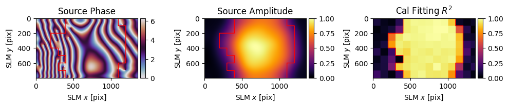
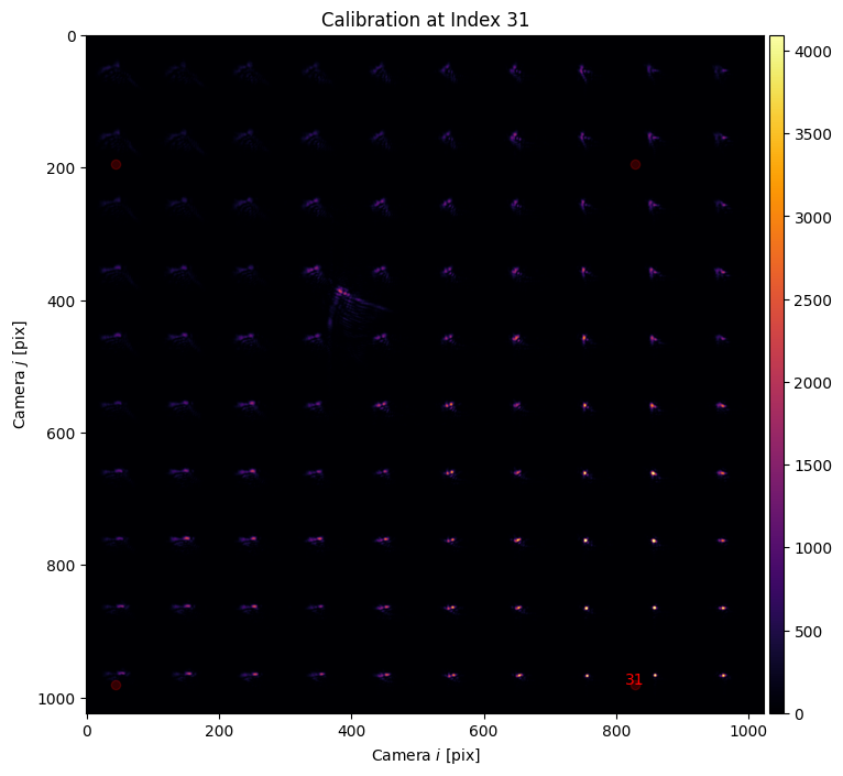
However, the analysis and smoothing uses the same method as single-point calibration, with the addition of the parameter index= to select which point of calibration is used. We don’t (currently) have a way to simulate varying aberration across the field of view, so if you’re running virtual hardware you will observe the same aberration at each point.

While the wavefront correction phase might look similar for each corner point, the resulting spot array only shows tightly focused spots in a patch around the point of correction. The next section will use techniques from previous tutorials and an alternative form of wavefront correction to recover good spots across the field of view.

Zernike Wavefront Calibration

Let’s start by removing the phase calibration applied to the SLM in the previous section so we can work from the start without correction.

if "phase" in slm.source: del slm.source["phase"]
if "wavefront_superpixel" in fs.calibrations: del fs.calibrations["wavefront_superpixel"]
if "wavefront_zernike" in fs.calibrations: del fs.calibrations["wavefront_zernike"]

We can make use of the Zernike spot optimization explored in the previous example to directly and iteratively remove aberration from every spot. The function .wavefront_calibrate_zernike() accepts vectors in Zernike-space, such that the user can provide an arbitrary set of points to correct or further-correct. We first need to build these vectors in Zernike-space 'zernike' from camera coordinates 'ij'.

from slmsuite.holography.toolbox import convert_vector

points_ij = fs.wavefront_calibration_points(pitch=75)

points_zernike = convert_vector(
    points_ij,
    from_units="ij",
    to_units="zernike",
    hardware=fs
)

This calibration scheme works by sweeping the addition of a Zernike term to the spot array, fitting to find the perturbation that realizes tight spots according to a figure of merit (defaults to spot area analysis.image_areas). Then the calibration iteratively subtracts the perturbation from the coordinate of the spot in Zernike-space.

We can test the Zernike wavefront calibration settings without starting an optimization step by using perturbation=0. Note that we also use the plot=2 flag to plot zoomed in windows on our array of spots.

fs.wavefront_calibrate_zernike(points_zernike, perturbation=0, plot=2);

The zernike_indices= argument allows the user to either say the desired Zernike basis (list) or ask for a number of (non-piston) Zernike terms (int). The 2D vectors that we’re providing are assumed to be the \(x,y\) terms and the vectors are zero-padded to include another 25 terms in Zernike-space, for the 27 indices that we request.

The perturbation= argument determines the size of our sweep in radians. For this SLM, with small anisoplanatism and larger global aberration, we first want to get an accurate starting point guess.

We’ve found that the first steps of optimization tend to work better if one first removes the shared aberration between all the spots with global_correction=True.

fs.wavefront_calibrate_zernike(
    points_zernike,
    zernike_indices=27,
    perturbation=np.linspace(-4*np.pi, 4*np.pi, 21, endpoint=True),
    global_correction=True,
    plot=False
);

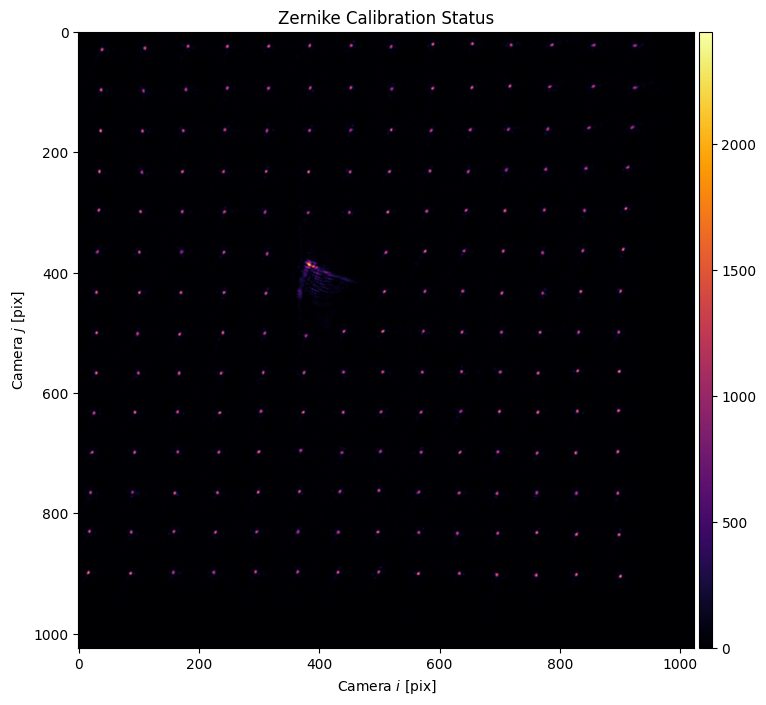
Our global correction finds a decent average wavefront correction pattern and recovers decent spots across most of the center of the plane.

fs.wavefront_calibrate_zernike(None, perturbation=0, plot=2);

Let’s refine this globally for one more step before turning to individual calibration.

fs.wavefront_calibrate_zernike(None, perturbation=np.pi, global_correction=True, plot=False);

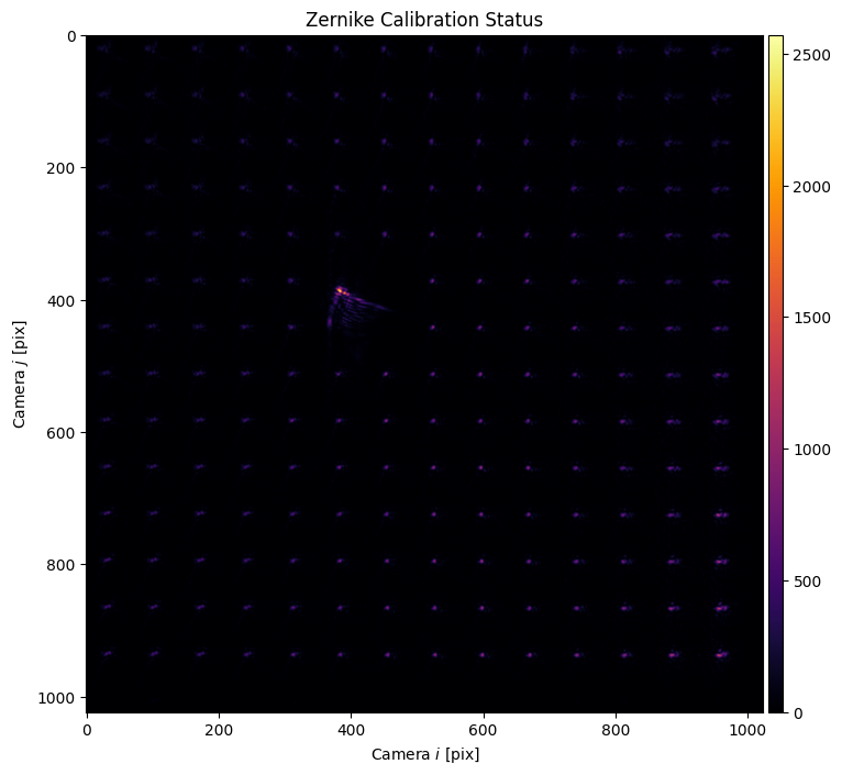
And then we again take a look:

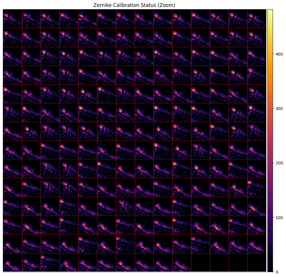
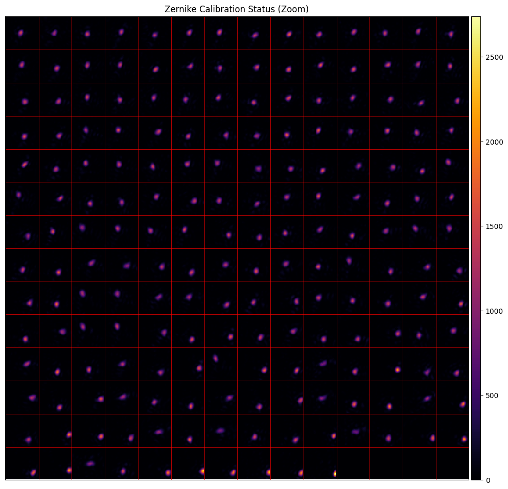
fs.wavefront_calibrate_zernike(None, perturbation=0, plot=2);

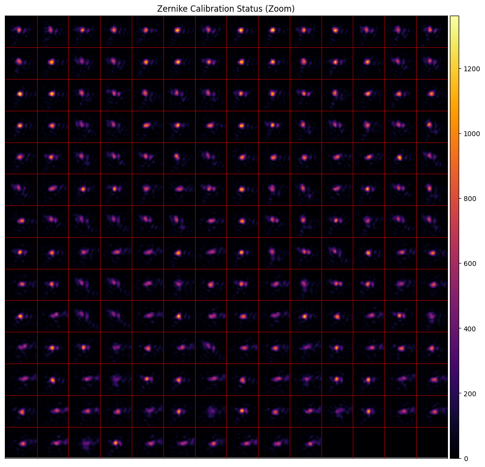
Now let’s move onto individual calibration, without the global_calibration flag.

fs.wavefront_calibrate_zernike(None, zernike_indices=27, perturbation=np.pi, plot=False);

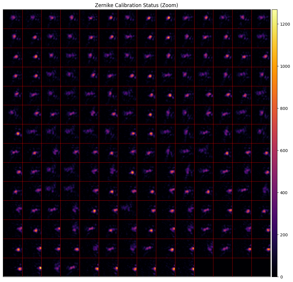
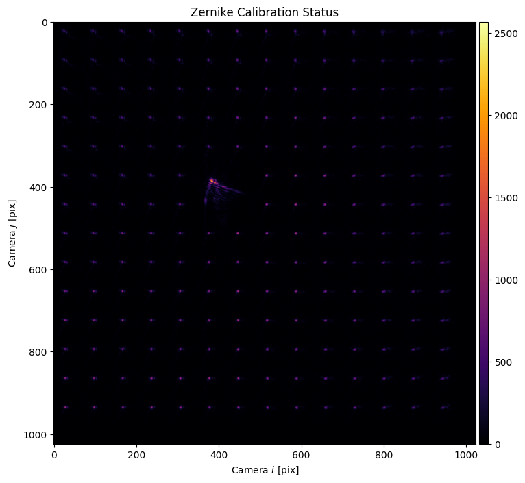
We expect the results to be a bit noisier because the correction is averaged over fewer points, but to also be a better correction on average as it accounts for anisoplanatism.

fs.wavefront_calibrate_zernike(None, perturbation=0, plot=2);

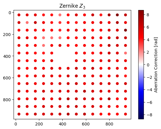
And this is what we find. We’re getting closer to good results. Here’s the measured strength of one term of aberration across the field of view, for instance. However, the noise is apparent, with occasional local outliers.

fs._wavefront_calibrate_zernike_plot_raw(index=3)

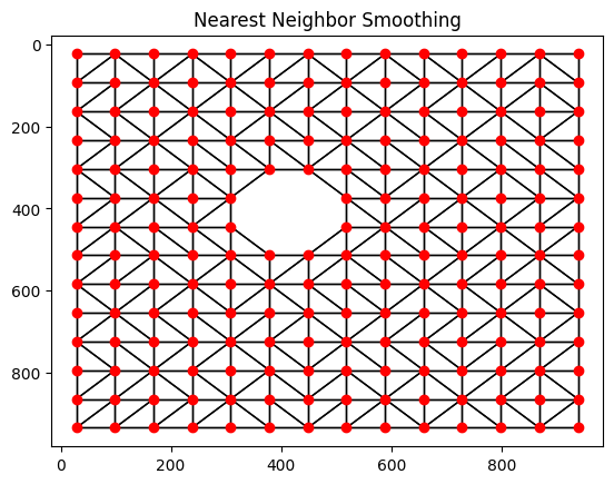
In order to account for some of the noise, we can assume that the aberration is locally smooth and average nearest neighbors via a helper function.

zernike_smoothed = fs.wavefront_calibrate_zernike_smooth(
    smoothing=0.5,
    smoothing_xy=0.5,
    plot=True
);

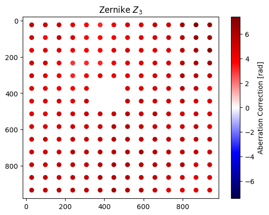
This smoothing reduces the prominance of some of the outliers.

fs._wavefront_calibrate_zernike_plot_raw(calibration_points=zernike_smoothed, index=3)

If we feed the smoothed data back into the calibration, we can see how it performs:

fs.wavefront_calibrate_zernike(zernike_smoothed, zernike_indices=27, perturbation=0, plot=2);

C:\Users\holodyne\Documents\GitHub\slmsuite\slmsuite\hardware\cameraslms.py:1974: UserWarning: Image might become overexposed during optimization (2740/4095).
  warnings.warn(

Overall, the spots are tighter, though they’re shifted around more. This is expected. Higher order Zernike terms have some contribution to local blaze, and as these are averaged, the tip tilt terms will need to be recentered. Our final steps of iteration will converge on a better and more centered result.

N = 4

for i in range(N):
    zernike_smoothed = fs.wavefront_calibrate_zernike_smooth(
        smoothing=0.5,
        smoothing_xy=0.5,
        plot=False
    )
    fs.wavefront_calibrate_zernike(zernike_smoothed, zernike_indices=27, perturbation=np.pi, plot=False)

As a final result, we find near-diffraction-limited spots across the field of view despite the anisoplanatic aberration.

fs.wavefront_calibrate_zernike(None, perturbation=0, plot=2);

C:\Users\holodyne\Documents\GitHub\slmsuite\slmsuite\hardware\cameraslms.py:1974: UserWarning: Image might become overexposed during optimization (2212/4095).
  warnings.warn(

Nice, tight spots.

It’s also important to mention that this method is quite general. .wavefront_calibrate_zernike() accepts user-provided functions to change the metric= of how spot images from the camera are judged, or completely change the heuristic by providing a custom callback=.

• The metric() takes in a stack of spot images, each image corresponding to one spot, and is respected to return a list of the goodness of each image.

• callback() overrides camera functionality and the user can choose how to determine the goodness. This, for instance, could be a measure of trap depth on atoms or similar measurement that avoids aberration between the camera and an experimental plane. After all, perfect spots on the camera might correspond to very distorted spots in an experimental plane.

MOreover, anisoplanatic aberration problem is exacerbated for high-NA setups where light is bent to a much larger degree than our simple <.1 NA setup does. As field of view sizes are pushed larger and larger, our software solution to compensating for aberration becomes increasingly important to close the gap between imperfect aberration mitigation engineered into the optical train and the ideal of aberration-free imaging.

Future additions to slmsuite will take greater advantage of this full-field calibration information. We look forward to seeing how far we can push this frontier!

slm.close()
cam.close()