Computational Holography

Before even connecting a physical spatial light modulator (SLM), slmsuite’s hardware simulation, modular iterative holography algorithms, GPU acceleration, and … suite … of toolboxes make it a powerful tool for computational holography education, exploration, and research.

In this first tutorial, we’ll walk through the basic functionality. Specifically, we will:

• Understand the connection between the SLM’s nearfield and farfield

• Program and visualize various target farfield patterns (spot arrays)

• Solve for the associated nearfield phase masks using iterative Fourier transform (e.g. Gerchberg-Saxton or “GS”) algorithms

• Compare convergence and pattern uniformity with various flavors of GS

• Generalize these principles from spot arrays to images

SLM Fundamentals

How do we steer light? A simple example is to use a mirror (see a, below) which steers the angle \(\theta\) of a beam in the farfield. Phase-mode spatial light modulators are displays whose pixels delay the wavefront of light. SLMs can therefore accomplish the same exact action of a tilted mirror by applying a linear shear to the display (see b). Hardware limitations (which limit achievable delays to order \(2\pi\)) usually necessitate that this phase is wrapped in the manner of a fresnel lens such that a larger tilt (i.e., phase gradient) can be applied on the display. The nearfield is related to the farfield by the Fourier transform, an inherent property of free-space propagation, so this linear shear in phase corresponds to the expected shift in the farfield (see c). We often think of the farfield as the ‘\(k\)-space’, or the space comprising of beams of light propagating along vectors \(\vec{k}\) at infinity. Here, we often use normalized units $ \begin{align} k_x = \frac{\vec{k} \cdot \hat{x}}{|\vec{k}|} \end{align} $ which are equivalent to \(\theta\) under the small angle approximation under which SLMs usually operate (the maximum steering range \(\theta = \lambda/\Lambda\) is on the order of a few degrees for common pixel pitches \(\Lambda\sim 10 \lambda\)). In b and c of the animation, for example, the SLM steers to the time-varying target angle \(k'_x\) in the far-field. Even though we depict the farfield pattern as an infinitely narrow \(\delta\) function, the true spot width \(\delta k'_x = 1/L\) for the aperture size \(L = N\Lambda\) is governed by the diffraction limit.

These principles readily extend to steering in two dimensions as illustrated in d and e.

Propagating to infinity (and even sometimes to the true farfield requirement \(z\sim L^2/\lambda\) for an SLM aperture dimension \(L\)) is a lot to ask of an experimental setup, so we can alternatively use a lens to focus the farfield pattern to an imaging plane. The simplest setup for a phase-type (e.g. LCOS) SLM places the device one focal length (\(f\)) in front of a lens to produce a desired image or pattern in the conjugate focal plane (i.e. the imaging plane a distance \(f\) behind the lens). In this common configuration, the lens counteracts the parabolic farfield focal plane such that the the SLM and imaging plane are ideally related by the Fourier transform (unfortunately, various types of aberration often stymie this).

More complicated setups (e.g., microscopes) often use systems of lenses; however, the power of the imaging system can still be distilled into some effective focal length \(f\). This \(f\) can be used to calculate a number of useful experimental properties of the system:

• For a beam steered along a given \(k_x\), the position in the imaging plane is \(X = k_xf\). Future tutorials will show how slmsuite automatically measures \(f\) to calibrate transformation between nearfield and farfield positions.

• For an SLM with pixel pitch \(\Lambda\), the Nyquist-limited edge of the farfield (the field of view of the SLM) is \(k_\text{max} = \pm\frac{\lambda}{2\Lambda}\) corresponding to \(X_\text{max} = \pm\frac{\lambda f}{2\Lambda}\). Such a pattern corresponds to the phase pattern \(\cdots 0, \pi, 0, \pi, 0, \pi, \cdots\) though by symmetry this pattern deflects power to both the positive and negative orders.

slmsuite handles much of this internally. We will next explore the relationship between the nearfield and farfield using slmsuite.

Beam Steering in slmsuite

We’ll start by importing slmsuite and a few packages. Note that slmsuite will automatically import `cupy <https://cupy.dev/>`__ for GPU acceleration if it’s installed; otherwise, numpy will be used for (slower) CPU-based computation.

We can use slmsuite’s phase retrieval algorithms to solve for the unknown nearfield phase pattern (that we’ll eventually apply to our SLM in an experiment) that reproduces the desired farfield target in the imaging plane. Let’s try it out with a simple farfield pattern: a single target pixel illuminated on a \(32 \times 32\) pixel grid.

# Import phase retrieval algorithms
from slmsuite.holography.algorithms import Hologram

# Make the desired image: a random pixel targeted in a 32x32 grid
target_size = (32, 32)
target = np.zeros(target_size)
target[9, 24] = 1

# Initialize the hologram and plot the target
# Note: For now, we'll assume the SLM and target are the same size (since they're a Fourier pair)
slm_size = target_size
hologram = Hologram(target, slm_shape=slm_size)
zoombox = hologram.plot_farfield(source=hologram.target, cbar=True)

In this case, we plotted the target in the basis "knm" representing the pixel indices of the SLM’s computational \(k\)-space (here, "knm" is aligned with the farfield camera’s pixels – the "ij" basis – so the two are synonymous). However, since this plane and the SLM plane are a Fourier pair, each target pixel corresponds to a 2D spatial frequency applied in the SLM plane. The exact unit conversion requires some physical properties of the SLM and camera (i.e., the detector imaging the farfield). To illustrate this point, we’ll instantiate simulated objects of the SLM and camera classes.

For our computations, these objects are just useful ways to store the simulated SLM and camera properties. In a real experiment, their methods will also control the hardware.

We’ll also instantiate a setup object (of the CameraSLM class) to store both the camera and SLM. In an actual experiment, the CameraSLM methods help find the relative orientation between the two devices (and more..).

# Create a virtual SLM and camera
from slmsuite.hardware.slms.simulated import SimulatedSLM
from slmsuite.hardware.cameras.simulated import SimulatedCamera
from slmsuite.hardware.cameraslms import FourierSLM

# Assume a 532 nm laser
wav_um = 0.532
slm = SimulatedSLM((slm_size[1], slm_size[0]), pitch_um=(10, 10), wav_um=wav_um)
camera = SimulatedCamera(slm)

# The setup (a FourierSLM setup with a camera placed in the Fourier plane of an SLM) holds the camera and SLM.
setup = FourierSLM(camera, slm)
hologram.cameraslm = setup

c:\Users\holodyne\Documents\GitHub\slmsuite-examples\examples\../../slmsuite\slmsuite\hardware\cameras\camera.py:444: UserWarning: 'camera' _get_image_hw() failed 5 times before quitting.
  warnings.warn(f"'{self.name}' _get_image_hw() failed {failures} times before quitting.")

With these objects created, we can now re-plot the target image plane in various spatial frequency units. See the slmsuite.holography.toolbox.convert_vector function documentation for definitions of these units.

# Not all inclusive, but try out a few units
for units in ["kxy", "freq", "deg"]:
    hologram.plot_farfield(source=hologram.target, units=units, figsize=(6,3))

With a solid understanding of the near- and farfield characteristics, we can now move onto actually solving for the nearfield phase mask. We’ll start with the classic Gerchberg-Saxton iterative Fourier transform algorithm.

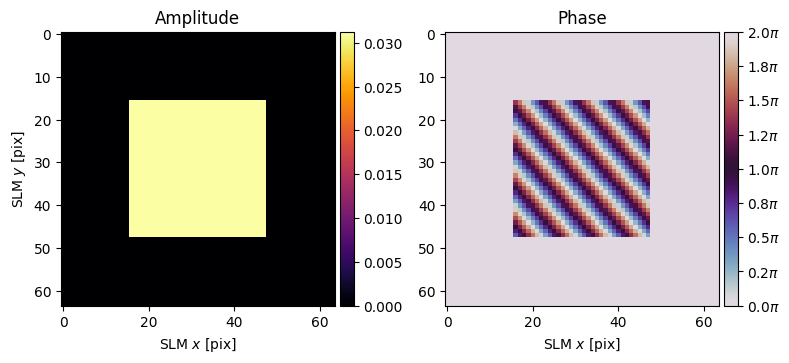
# Run 5 iterations of GS.
hologram.optimize(method='GS', maxiter=5)

# Look at the associated near- and far- fields
hologram.plot_nearfield(cbar=True)
hologram.plot_farfield(limits=zoombox, cbar=True, title='FF Amp');

The nearfield amplitude is unity (the SLM class assumes uniform illumination by default) and GS calculated a beautiful diagonal grating with a ~4 pixel horizontal/vertical period as expected from the unit conversion plots above (see the "freq" unit conversion plot, where \(1/f_x\sim 1/f_y\approx 1/4\)).

While at first glance it looks like the GS-computed phase mask exactly reproduces the desired farfield target pattern, this is actually not the case. From basic Fourier theory, we know that a uniformly illuminated aperture (comprising \(N\) pixels at pitch \(\Lambda\) will emit a beamwidth \(\delta k_x \approx \lambda/N\Lambda\)). Sampling in increments of \(\Lambda\) in the nearfield also corresponds to a total spatial frequency range of \(\lambda/\lambda{\Lambda}\), which yields a bin width \(\lambda/N\Lambda\) for \(N\) pixels. So it only appears that we created the perfect target pattern because each pixel in the farfield corresponds to a diffraction-limited spot.

To see the true pattern, we can increase the farfield resolution by zero-padding the nearfield.

from slmsuite.holography import toolbox

# Get the padding needed to resolve 2x smaller than a diffraction limited spot
# (N.b. slm.pitch, like all length variables in slmsuite, is wavelength-normalized)
hologram.shape = hologram.get_padded_shape(setup, precision=0.5/(slm.pitch[0]*slm.shape[0]))
target_padded = toolbox.pad(target, hologram.shape)

# Recompute the farfield
hologram = Hologram(target_padded, slm_shape=slm.shape)
zoombox_padded = hologram.plot_farfield(target_padded)
hologram.optimize(method='GS', maxiter=5)

# Look at the associated near- and far- fields
hologram.plot_nearfield(padded=True, cbar=True)
hologram.plot_farfield(cbar=True, units="deg", title='FF Amp', limits=zoombox_padded);

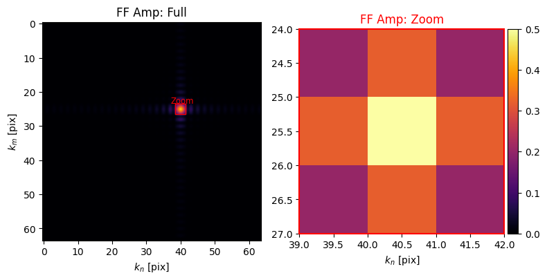
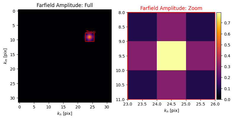
Likewise, farfield pixels are also smaller than diffraction limited spots when the nearfield amplitude doesn’t fully fill the SLM aperture as illustrated below.

# Set a Gaussian amplitude profile on SLM
slm.set_source_analytic()   # With no arguments, defaults to a beamradius equal to half the aperture size

# Redo the same GS calculations
hologram = Hologram(target, slm_shape=slm.shape, amp=slm.source["amplitude"])
hologram.optimize(method='GS', maxiter=5)

hologram.plot_nearfield(padded=True,cbar=True)
hologram.plot_farfield(cbar=True,limits=zoombox);

Spot Arrays

Now that we’ve discussed bare-bones GS algorithms, SLM setups, and Fourier principles, we can move onto more realistic targets. Here, for example, we’ll start looking at many spots in the target plane instead of a single one. These patterns may seem simple but are actually an enabling tool for state-of-the-art quantum computing (where arrays of optical tweezers – the topic of the 2018 Nobel Prize in Physics – trap and excite atom arrays), optogenetics (where desired neurons are dynamically excited), and laser printing.

Let’s give it a shot with SpotHologram, a child of the Hologram “super-class” with various utilities for making and characterizing spot arrays.

from slmsuite.holography.algorithms import SpotHologram

# Move to a larger grid size
slm_size = (1024, 1024)

# Instead of picking a few points, make a rectangular grid in the knm basis
array_holo = SpotHologram.make_rectangular_array(
    slm_size,
    array_shape=(10,10),
    array_pitch=(10,10),
    basis='knm'
)
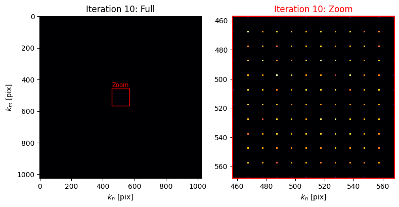
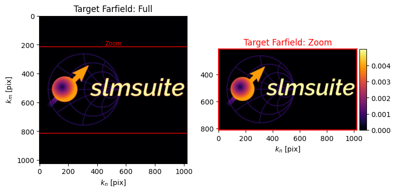
zoom = array_holo.plot_farfield(source=array_holo.target, title='Target Farfield')

Now we’ll run the optimization to produce our intended target: a farfield array of optical foci with uniform amplitude). For ease, the optimize method uses a parameter naming convention borrowed from `scipy.optimize <https://docs.scipy.org/doc/scipy/reference/optimize.html>`__. It’s therefore simple enough to add a callback funtion that runs during each iteration of GS, which we demonstrate below.

# Example callback function: plot the FF every 10 iterations
def plot_ff(holo):
    if holo.iter % 10 == 0:
        holo.plot_farfield(limits=zoom, title='Iteration %d'%holo.iter)

# Now we'll run the computation using 21 iterations of GS.
array_holo.optimize(method="GS", maxiter=21, callback=plot_ff,
                    stat_groups=['computational_spot'], verbose=False)

We see here that GS converges within a few steps to an image close to our target pattern. But how close? In the cell above, the addition of the stat_groups=['computational'] parameter to the optimization loop had dual purpose: it 1) calculated statistics of the spot array uniformity and efficiency at each step of the GS optimization which 2) forced array_holo.amp_ff to be computed so that we could plot it with our callback function (for speed, amp_ff is not calculated at each optimization step unless needed).

Sidenote: statistics computation slows down GS (due to data transfer between numpy and cupy objects during each GS iteration) but has been heavily optimized to limit the performance loss.

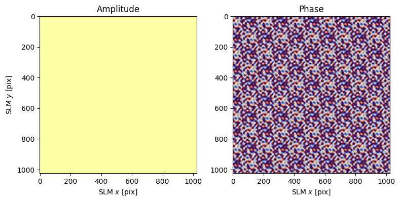
We can now plot the algorithm convergence (to see “how close” we got to the target) and the final nearfield phase mask produced by the algorithm.

array_holo.plot_stats()
array_holo.plot_nearfield()

Comparing Algorithms

For the default GS algorithm, the inefficiency (fraction of power off-target), non-uniformity, and associated amplitude errors converge within a handfull of optimization iterations. The 50% resulting non-uniformity isn’t stellar. Fortunately, a number of other “weighted” (i.e. “WGS”) GS algorithms can improve these results.

A complete listing of implemented algorithms can be found in the `slmsuite documentation <https://slmsuite.readthedocs.io/en/latest/index.html>`__. Here, we’ll use a recently-developed fixed-phase WGS algorithm to compare to basic GS.

# Retry with WGS using a fixed-phase algorithm
import copy

wgs_holo = copy.deepcopy(array_holo)
wgs_holo.reset()
wgs_holo.optimize(method="WGS-Kim", maxiter=21,verbose=2, stat_groups=['computational_spot'])
wgs_holo.plot_farfield(limits=zoom);

Optimizing with 'WGS-Kim' using the following method-specific flags:
{'feedback': 'computational',
 'feedback_exponent': 0.8,
 'fix_phase_efficiency': None,
 'fix_phase_iteration': 10}

Since we included verbose=2 argument in the optimize call, we also see the flags being used by the optimization algorithm. Default values are assigned in slmsuite but you can pass any of these flags as an optimize argument to change the algorithm behavior (the stat_groups list is one example shown here).

Let’s now compare the results.

# Combine the statistics and compare
statscombined = wgs_holo.stats
statscombined["stats"]['WGS'] = statscombined["stats"].pop("computational_spot")
statscombined["stats"]["GS"] = array_holo.stats["stats"]["computational_spot"]

# (Optional) Reverse order to plot GS first
statscombined["stats"] = dict(reversed(list(statscombined["stats"].items())))

ax = wgs_holo.plot_stats(statscombined)

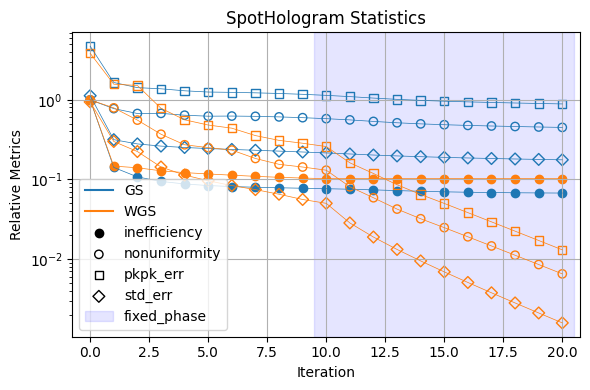
Much better: the WGS algorithm quickly converges once the farfield phase is fixed (defined here by the WGS-Kim algorithm’s default fix_phase_iteration=10 setting) at the cost of a slight efficiency reduction.

Basic Image Formation

The same algorithms can be applied to more complex patterns, like pictures. Notice that the image is very good, but not perfect. This is because perfect nearfield phase retrieval is impossible in general for a fixed nearfield amplitude distribution (in our case, the amplitude is uniform by default).

import cv2

# Use a random logo
path = os.path.join(os.getcwd(), '../../slmsuite/docs/source/static/slmsuite-small.png')
img = cv2.imread(path, cv2.IMREAD_GRAYSCALE)
img = cv2.bitwise_not(img) # Invert
assert img is not None, "Could not find this test image!"

# Resize (zero pad) for GS.
shape = (1024,1024)
target = toolbox.pad(img, shape)

holo = Hologram(target)
zoom = holo.plot_farfield(holo.target, cbar=True, title='Target Farfield')

holo.optimize(method="WGS-Kim", maxiter=21)
holo.plot_farfield(limits=zoom,title='WGS Image Reconstruction', cbar=True)
holo.plot_farfield(np.abs(holo.target - holo.amp_ff), limits=zoom, title='WGS Image Error', cbar=True);

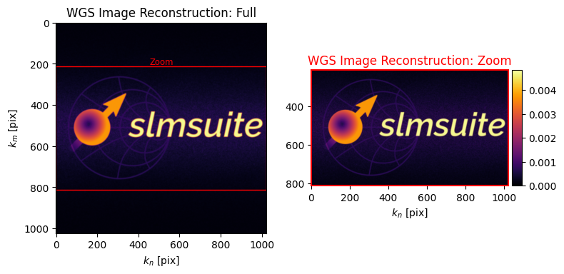
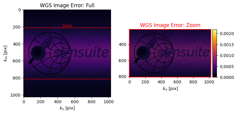
We’ll return to image formation in the experimental holography tutorial.

Future Development

Notice that none of the examples in this notebook took more than 1 second to run: slmsuite is fast. In the future, we plan to add more algorithms (e.g., gradient descent-based amplitude and phase reconstructions) and full experimental simulation to assist in the development of new SLM algorithms and techniques. We hope that you’ll join us!