

Wavefront Calibration#
Thus far, our examples have made two important assumptions:
The SLM is perfectly in the Fourier domain without aberration (connected to the imaging domain via an ideal Fourier transform)
The optical amplitude of the source beam covers the SLM uniformly.
Generally, in practical experiments, both assumptions are false.
Beamline misalignment, defocus, or imperfect optics will cause optical aberration.
The source beam will generally be Gaussian, and cannot cover the SLM uniformly without significant loss.
In this example, we will make use of functions and calibrations built into slmsuite to:
Correct for optical aberration, such that phase profiles can be displayed with compensation, and
Measure the sourced amplitude, such that GS-type optimization algorithms use a better base approximation the system (see
slmsuite.holography.algorithms).
Initialization#
To start, we initialize our system consisting of a camera and a SLM separated by a Fourier transform.
[23]:
# Try to load physical hardware.
try:
    from slmsuite.hardware.slms.texasinstruments import PLM
    from slmsuite.hardware.cameras.flir import FLIR

    # Load the hardware.
    slm = PLM('p67', 1, wav_um=0.488, settle_time_s=0.05, configure_usb=True); print()
    cam = FLIR(serial="22562470", pitch_um=2.74, bitdepth=12)

    # For this camera, we also want to crop the WOI to the center 1024x1024 area.
    h_max, w_max = cam.default_shape
    cam.set_woi(((w_max - 1024) // 2, 1024, (h_max - 1024) // 2, 1024))

    # Load the composite CameraSLM.
    fs = FourierSLM(cam, slm)
# Fallback to virtual hardware.
except Exception as e:
    print(f"Loading physical hardware failed; loading virtual hardware. Error:\n{str(e)}")
    from slmsuite.hardware.slms.simulated import SimulatedSLM
    from slmsuite.hardware.cameras.simulated import SimulatedCamera

    # Make the SLM and camera.
    slm = SimulatedSLM((1600, 1200), pitch_um=(8,8))
    from slmsuite.holography.toolbox.phase import zernike_sum
    phase_aberration = zernike_sum(
        slm,
        indices=(3, 4, 5, 7, 8),
        weights=(1, -2, 3, 1, 1),
        aperture=None,
        use_mask=False
    )
    slm.set_source_analytic(                        # Program the virtual source.
        phase_offset=phase_aberration,
        sim=True
    )
    slm.plot_source(sim=True)

    cam = SimulatedCamera(slm, (1440, 1100), pitch_um=(4,4), gain=200)

    # Tie the camera and SLM together with an analytic calibration.
    fs = FourierSLM(cam, slm)
    M, b = fs.fourier_calibration_build(
        f_eff=80000.,                              # f_eff of 80000 wavelengths or 80 mm with the default 1 um wavelength
        theta=5 * np.pi / 180,
    )
    cam.set_affine(M, b)
    fs.fourier_calibrate_analytic(M, b)
PLM using GPU (cupy) backend
DLPC900 connected: firmware {'app_version': 95, 'api_version': 72, 'sw_patch': 111, 'sw_minor': 108, 'sw_major': 111}
DLPC900 pre-configured (video mode, display detected)
Initializing pyglet... success
Searching for window with display_number=1... success
Creating window... Window creation successful
DLPC900 source locked, switching to video-pattern mode...
DLPC900 configured successfully - pattern sequence running

Looking for cameras... PySpin sn '22562470' initializing... PixelFormat set to Mono16 (12-bit)... Frame rate set to 33.7 Hz... Successfully initialized FLIR cam 22562470.
For this tutorial, we’re setting the calibration exposure for our setup. Users should tune in this to nicely expose their patterns.
[24]:
cam.set_exposure(.04);
We also make a helper function which we will use to display results:
[25]:
single_spot_exposure = 29e-6

def plot(title="", cam_limits=.25):
    old_exposure = cam.get_exposure()
    cam.set_exposure(single_spot_exposure)

    _, axs = plt.subplots(1, 2, figsize=(16,6))
    plt.sca(axs[0]); fs.slm.plot(slm.phase, title="Displayed Phase", cbar=True)
    plt.sca(axs[1]); fs.cam.plot(title="Camera Result", limits=cam_limits, cbar=True)
    plt.suptitle(title)
    plt.tight_layout()
    plt.show()

    cam.set_exposure(old_exposure)
Without Wavefront Calibration#
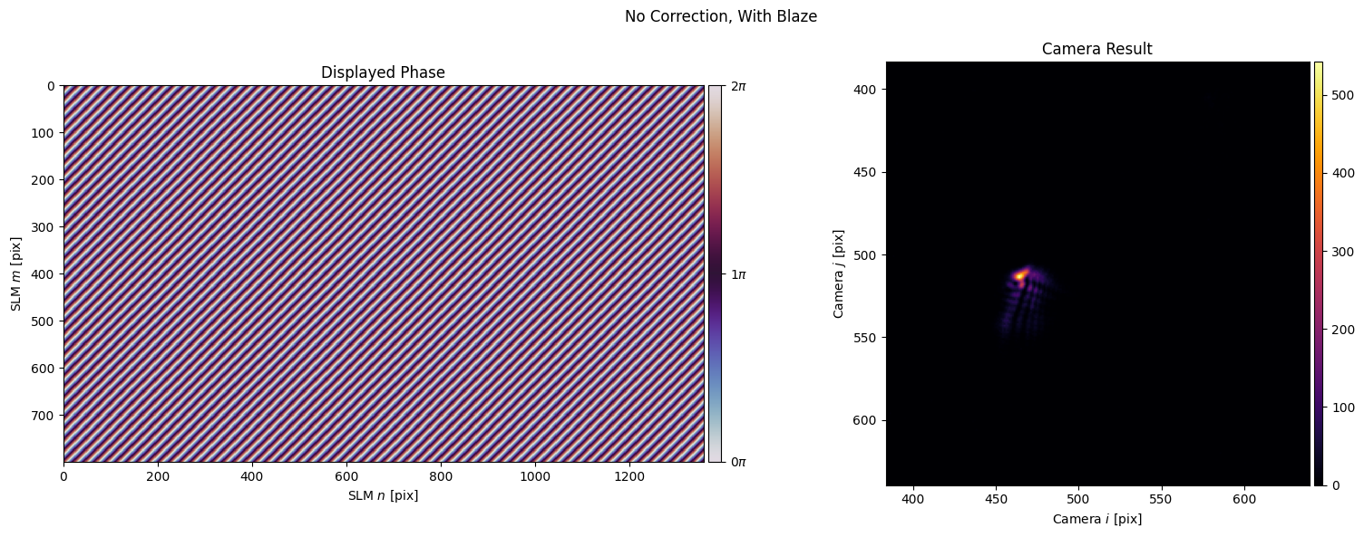
An uncalibrated SLM will generally not achieve diffraction-limited performance. For instance, some SLMs possess inherent curvature, which must be calibrated for ideal operation. We can take a look at this aberration:
[26]:
slm.set_phase(None, settle=True)
plot(title="No Correction, No Blaze")

slm.set_phase(blaze(grid=slm, vector=(.002, .002)), settle=True)
plot(title="No Correction, With Blaze")

With Vendor Phase Calibration#
Some vendors provide phase calibration data for the wavefront of their SLMs, usually acquired by Shack-Hartmann wavefront sensing. Subclasses implementing a vendor’s SDK can also support the SLM.load_vendor_phase_calibration() function to interpret the file provided by the vendor (.csv in the case of Santec). Unfortunately, we didn’t have this information for our SLM so we here leave the example code commented
out.
[27]:
# slm.load_vendor_phase_correction(
#     file_path='Wavefront_correction_Data_221136000005(830nm).csv',  # Update this path to load your calibration
#     smooth=True
# )
Still, we can often do better. The vendor-provided data only corrects for aberration on the SLM, but does not know about other beamline aberrations related to our setup. Additionally, information regarding source amplitude is valuable for holography. Calibrating these values, as aforementioned, is the goal of FourierSLM.wavefront_calibrate().
Fourier Calibration#
The automated wavefront calibration routines which are part of slmsuite are conducted through camera feedback. For this to work, we first need to calibrate the camera’s Fourier domain (see Experimental Holography). Note that in this case, it is critical to apply some form of phase correction before calibrating, as otherwise the spots in the Fourier calibration grid would be sufficiently diffraction limited to resolve a grid.
[28]:
fs.fourier_calibrate(
    array_shape=20,                 # Size of the calibration grid (Nx, Ny) [knm]
    array_pitch=20,                 # Pitch of the calibration grid (x, y) [knm]
    plot=True
);
C:\Users\holodyne\Documents\GitHub\slmsuite\slmsuite\holography\toolbox\__init__.py:258: UserWarning: CameraSLM must be passed as slm for conversion 'kxy' to 'ij'
  warnings.warn(

Testing Wavefront Calibration#
Now we are ready for wavefront calibration. This is a serial process where ‘superpixels’ on the SLM of size superpixel_size\(\times\)superpixel_size pixels are tested one after another. We are looking to measure, as mentioned in the introduction, two things:
A local phase correction factor about each superpixel, to counteract optical aberration, and
A measurement of the optical amplitude at each superpixel.
We can measure these by:
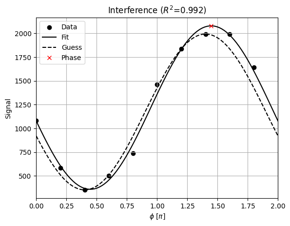
Interfering a given superpixel with some reference superpixel (chosen by default to be at the center of the SLM). A fit to the resulting interference fringes yields a measurement of the phase correction needed to bring the given superpixel into the same Fourier plane as the reference superpixel.
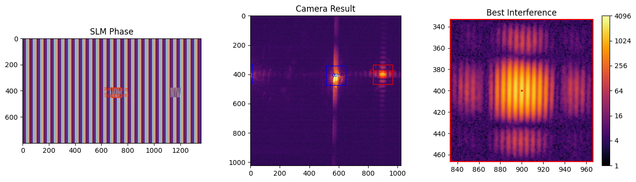
Integrating the power (amplitude squared) confined in the diffraction order corresponding to the superpixel.
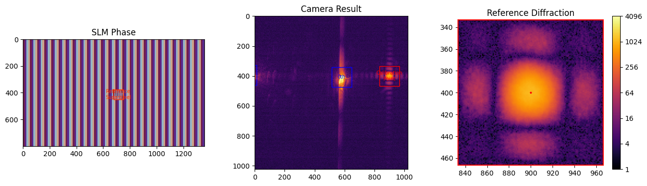
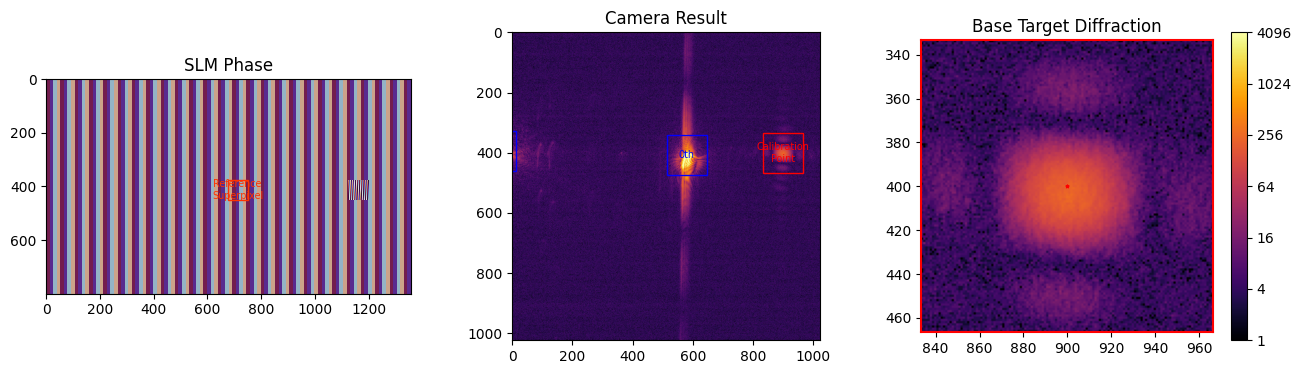
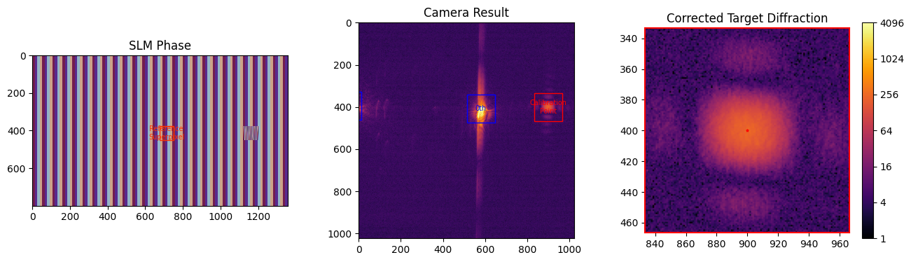
FourierSLM.wavefront_calibrate() is designed with a testing feature, such that when the test_index keyword is passed, the user is provided with helper plots to make sure that calibration is working at the superpixel corresponding to test_index. Shown below is the result for the superpixel with index 5: the 5th step in the wavefront calibration’s sweep. If one looks closely at the phase, small square superpixels can be seen where power is diffracted into a different order. Note
the titles of the plots which explain the purpose of each step in this process. The final returned dictionary contains the data that will be gathered from each superpixel on the SLM.
We’re also going to activate a special mode (plot=3) to generate a .gif sweeping across the interference condition.
[29]:
movie = fs.wavefront_calibrate(
    calibration_points=(900, 400),
    field_point=(.25, 0),
    field_point_units="freq",
    superpixel_size=75,
    corrected_amplitude=True,
    test_index=5,                       # Testing mode
    phase_steps=10,                     # Step through phase for the .gif
    plot=3                              # Special mode to generate a phase .gif
)

from slmsuite.holography.analysis.files import save_image

save_image("wavefront.gif", movie, loop=0)
We use markdown to display the .gif we just made:

The diffracted spot resulting from these rectangular superpixels matches their Fourier transform: the amplitude of a rectangular sinc function.
Note that this function returns the result of calibration on a given superpixel, where 'power', 'normalization, and 'background' deal with parameters relevant to amplitude calibration, and other parameters—especially 'phase', 'kx', and 'ky'—are relevant for phase calibration.
Testing allows the user to hone parameters for more ideal calibration, specifically:
calibration_points, the point in the camera’s"ij"basis where interference takes place.As the plural implies,
slmsuitecan simultaneously calibrate at many points, but for this tutorial we just feed one point.The
calibration_pointsshould be far from sources of noise, especially the ordered diffraction peaks of the field which contain the vast majority of the optical power in the system.Wavefront calibration works best in a region around each of the
calibration_points. The extent of this region depends on the parameters of the optical system and the nature of the aberrations.
field_point, the point in the camera’s"ij"basis where the field (power not in a superpixel) is deflected towards.This is useful because it reduces the power in the 0th order. This should be chosen such that higher diffraction orders from the field are far away from the
calibration_points.
Camera exposure.
If the user does not use the
autoexposureparameter (which sets the maximum exposure of the camera to be 10% of the dynamic range), then the user should make sure that calibration does not overexposure the camera during the calibration process. This might involve trying differenttest_superpixelsuperpixels to test superpixels with higher or lower power.
superpixel_size, the size in SLM pixels of each superpixel.In general, this should be chosen to be a small as reasonable within SNR and time constraints.
Ideally, it would also be a divisor of both the width and height of the SLM, so there are no cropped superpixels.
test_index, which iteration to examine as a test (described above).Based on how the calibration is scheduled, small indices will generally yield interference superpixels that are close to the reference superpixel, which usually produces the brightest results if the SLM source is centered. This also provides an opportunity to check for overexposure.
Wavefront Calibration#
With calibration working on this test case, we proceed to do this process over the full SLM. Removing the test_superpixel keyword disables testing mode and begins a long serial process of testing each superpixel. tqdm bars monitor progress for user feedback (though these may not be visible in the final notebook).
[30]:
fs.wavefront_calibrate(
    calibration_points=(900, 400),
    field_point=(.25, 0),
    field_point_units="freq",
    superpixel_size=75
);
We should save the data immediately after this measurement.
[31]:
fs.save_calibration("wavefront_superpixel");
Processing Wavefront Calibration#
The raw data from wavefront calibration is stored and saved in a compressed form, where a few floating numbers are recorded for each superpixel. To use this data, we still need to process the information on a per-pixel basis, rather than per-superpixel. This is done by FourierSLM.process_wavefront_calibration(). There are a few options (among others) available to the user for honing calibration processing.
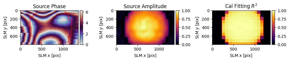
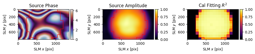
r2_thresholdsets the threshold for which bad fits are ignored. Notice below that there is significant clipping in the domain of the SLM. Within the clipped region, the fits are good, but outside it’s noise. The thresholdr2_thresholdcan be adjusted to omit or include superpixels at the user’s preference (boundary marked as red lines in the below plots). There are a few adaptive features to guess what the phase would look like in below-threshold superpixels.smoothadds blurring to the final result to smooth out the discretization caused by the superpixel approach. This will yield better results in practice as it avoids discontinuities between superpixels.
[32]:
# Without smoothing
fs.wavefront_calibration_superpixel_process(r2_threshold=.5, smooth=False, plot=True);
C:\Users\holodyne\Documents\GitHub\slmsuite\slmsuite\hardware\cameraslms.py:3720: UserWarning: remove_background is enabled and a noise floor was detected; removing this background (0.06709127128124237% of the average normalization).
  warnings.warn(
[33]:
# With smoothing
fs.wavefront_calibration_superpixel_process(r2_threshold=.8, smooth=True, plot=True, remove_background=True);
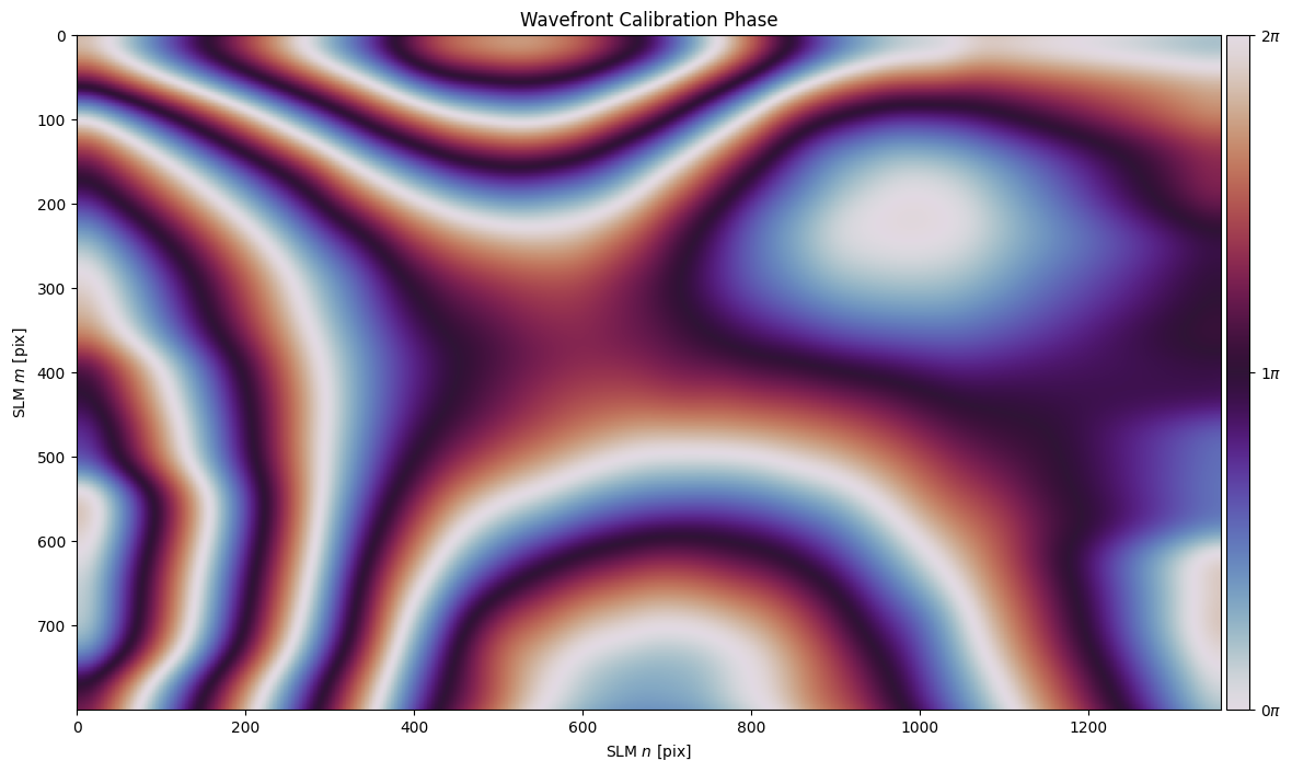
[34]:
# Make a plot for the thumbnail.
slm.plot(slm.source["phase"], title="Wavefront Calibration Phase");
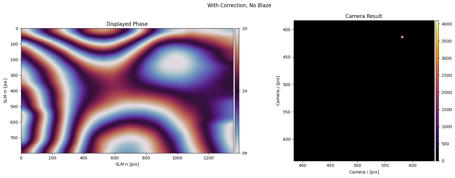
Now let’s revisit our plots from earlier. Instead of having a distorted spot, our power is far more concentrated!
[35]:
slm.set_phase(None, settle=True)
plot(title="With Correction, No Blaze")
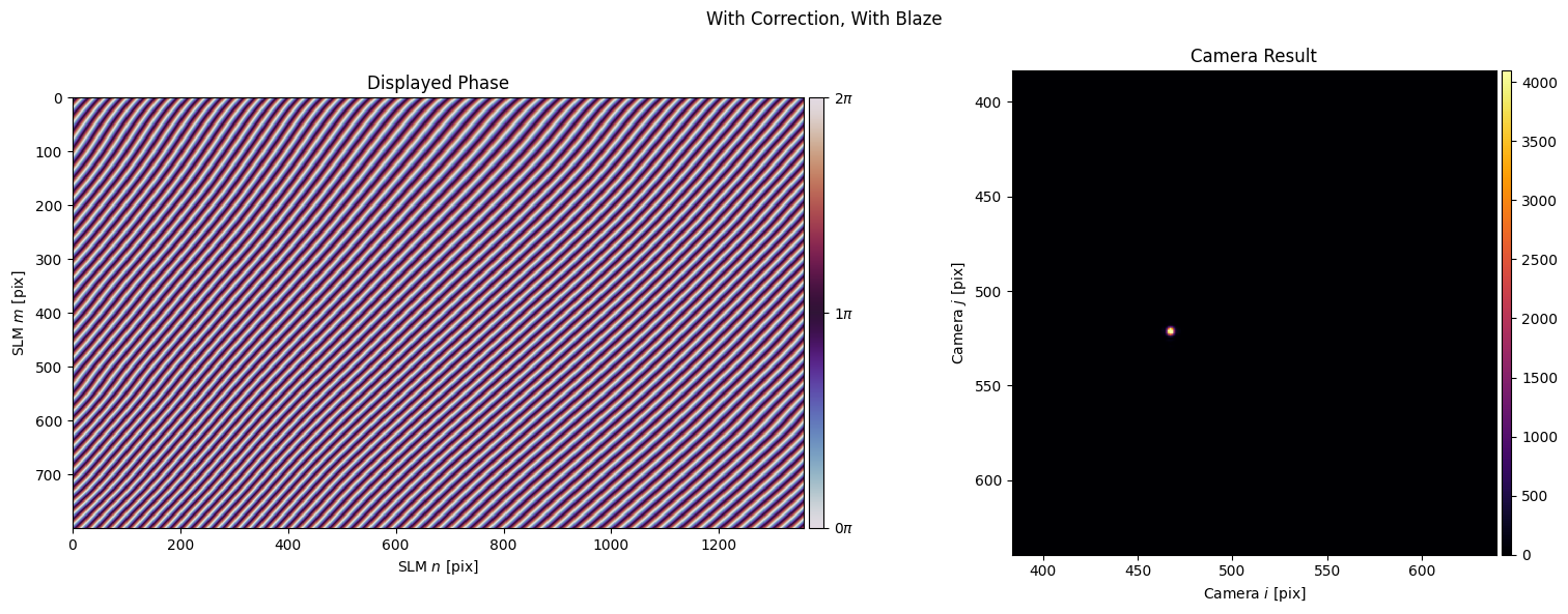
slm.set_phase(blaze(grid=slm, vector=(.002, .002)), settle=True)
plot(title="With Correction, With Blaze")
Re-Running Fourier Calibration#
Wavefront calibration will usually shift spot positions slightly due to net blaze in the calibration. This is mitigated to some extent with the remove_blaze=True parameter in wavefront_calibration_superpixel_process, but isn’t perfect due to higher order aberration terms with variable blaze over the aperture.
Thus, we suggest to re-run Fourier calibration after calibrating the wavefront. To this end, slmsuite will warn the user that the Fourier calibration is ‘stale’ if a newer wavefront calibration is detected during coordinate transformations.
[36]:
fs.ijcam_to_kxyslm([500, 500])
C:\Users\holodyne\Documents\GitHub\slmsuite\slmsuite\hardware\cameraslms.py:1373: UserWarning: The wavefront calibration is newer (2026-03-22 15:25:11.332053) than the Fourier calibration (2026-03-22 15:21:55.531875). The Fourier calibration may be stale.
  warnings.warn(
[36]:
array([[0.00138898],
       [0.00172398]])
Let’s save the calibration’s shift vector for comparison later.
[37]:
b_old = fs.calibrations["fourier"]["b"]
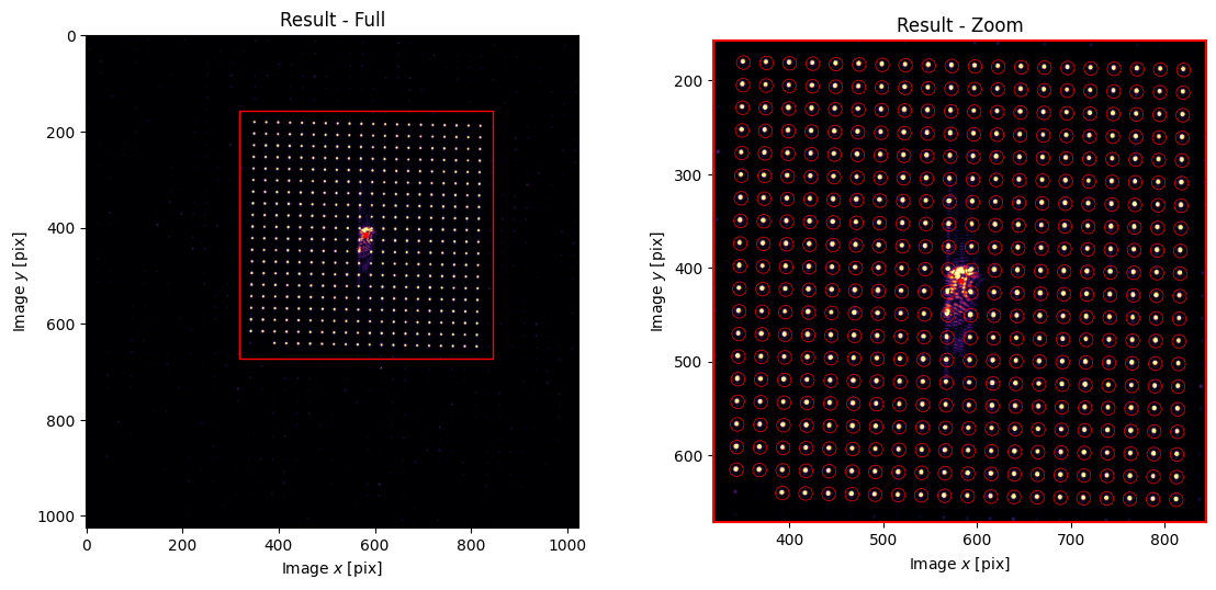
Performing Fourier calibration after the wavefront is calibrated also leads to a significantly cleaner spot array for fitting, compared to distorted pre-wavefront-calibration spots which could be mis-fit.
[38]:
fs.fourier_calibrate(
    array_shape=20,                 # Size of the calibration grid (Nx, Ny) [knm]
    array_pitch=20,                 # Pitch of the calibration grid (x, y) [knm]
    plot=True
);
Indeed, our Fourier calibration shifts by a few pixels after wavefront correction:
[39]:
b_new = fs.calibrations["fourier"]["b"]
b_new - b_old
[39]:
array([[2.00689562],
       [6.98383853]])
[40]:
slm.close()
cam.close()