

Experimental Holography#
slmsuite targets experimental holography on physical hardware. In this example, we show how to connect to a camera and an SLM and calibrate the transformation between the camera’s space and the SLM’s \(k\)-space.
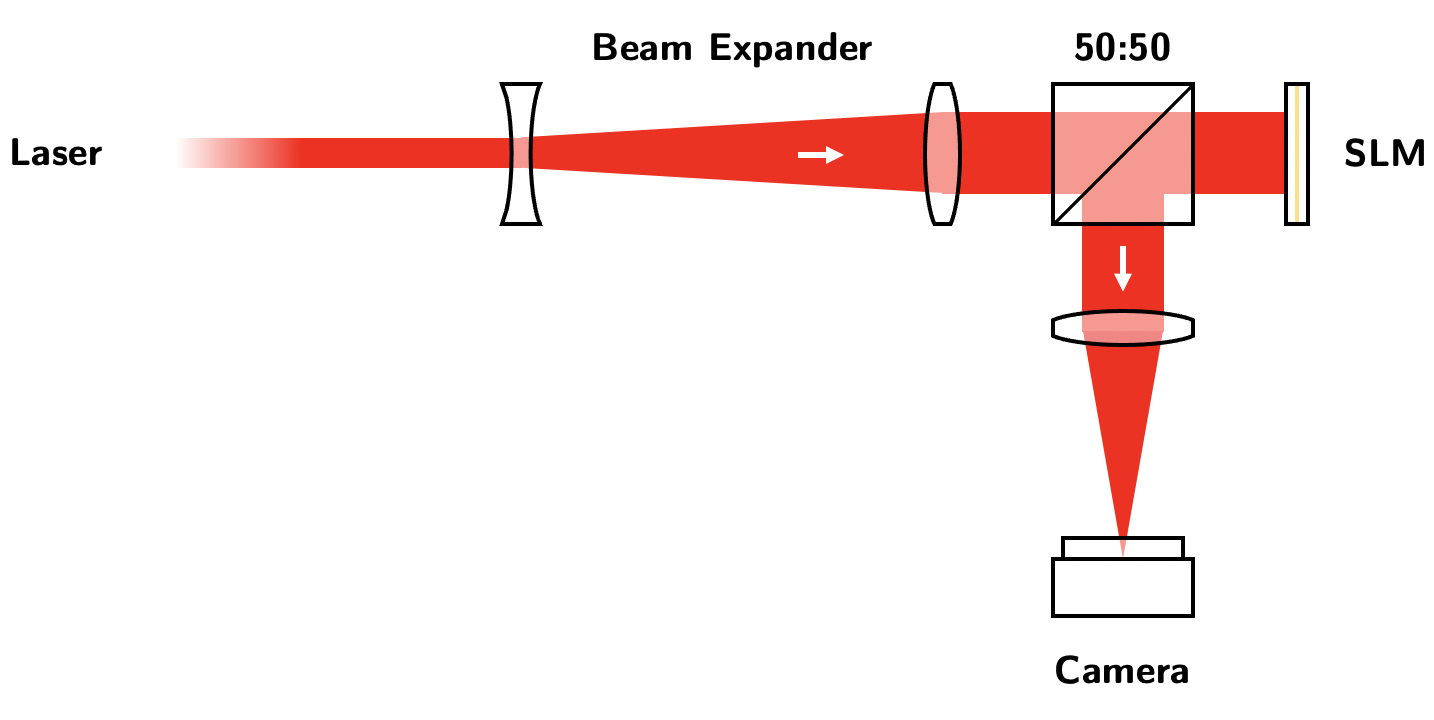
The setup running this notebook (and the notebooks for other examples) is very simple. From the left in the below diagram, we have an input laser which is expanded to the size of the SLM. This light reflects from the SLM, exits the alternate port of a 50:50 beamsplitter, and reaches the camera. Importantly, a lens is positioned inbetween the camera and SLM with a distance corresponding to the focal length \(f\) from each. Thus, the camera’s imaging plane is the farfield of the SLM (also called Fourier domain or \(k\)-space of the SLM). Note that this setup is simple, but is not necessarily optimal for a given application. Interrogating the SLM at a shallow angle, for instance, will avoid stray reflections and the 75% efficiency hit.
Loading Hardware#
Cameras and SLMs are connected to python by a myriad of SDKs, often provided by hardware vendors. However, these SDKs likewise have a myriad of function names and hardware-specific quirks. Thus, hardware in slmsuite is integrated as subclasses of the abstract classes .Camera and .SLM. These subclasses for cameras and
slms are effectively wrappers for given SDKs, implemented with standardized methods and syntax that the rest of slmsuite can understand, but also include quality-of-life features. SLMs that do not have a display SDK are often interfaced to via a virtual screen, and the ScreenMirrored class projects phase onto these. If you believe your camera or SLM is not supported by the currently available
classes, please open a GitHub issue or feel free to write an interface yourself using the provided templates!
First, let’s load an SLM. We’re running this notebook with a Texas Instruments Phase Light modulator, but this can be changed to any supported SLM or run with virtual hardware. Future notebooks explicitly try/except to fallback to run on virtual hardware if loading physical hardware fails. For clarity when introducing hardware loading, this notebook uses some documentation magic to hide the fallback code here (but the code is there if the notebook is loaded opened the docs).
For physical hardware implemented in slmsuite, we can detect connected interfaces with the .info() static method.
[136]:
from slmsuite.hardware.slms.texasinstruments import PLM
PLM.info();
Display Positions:
#,  Position
0,  x=0, y=0, width=1920, height=1080 (main)
Since our SLM is a ScreenMirrored SLM (i.e., the SLM mirrors a monitor on the local computer), the .info() method returns information about the local monitors. In our case, Display 0 is the main computer display, which we’re using to configure this notebook.
The PLM hasn’t been configured as a display yet via USB, so it doesn’t yet appear in this list. Our PLM USB configuration in the next cell takes care of this when we provide the display_number=1 argument (one-up count from the locally available displays). Other ScreenMirrored SLMs may already appear as displays without this extra configuration step.
[137]:
slm = PLM(display_number=1, model_name='p67', wav_um=0.488, settle_time_s=0.05, configure_usb=True)
PLM using GPU (cupy) backend
DLPC900 connected: firmware {'app_version': 95, 'api_version': 72, 'sw_patch': 111, 'sw_minor': 108, 'sw_major': 111}
DLPC900 pre-configured (video mode, display detected)
Initializing pyglet... success
Searching for window with display_number=1... success
Creating window... Window creation successful
DLPC900 source locked, switching to video-pattern mode...
DLPC900 configured successfully - pattern sequence running
We’ve given the class other important information:
The
model_nameof PLM we’re using,'p67', which loads the correct pixel size, resolution, and LUT.The wavelength
wav_umused in our system, here 488 nm laser. Combined with the pixel size, this calibrates unit conversions needed to run the SLM.The settle time in seconds of the SLM
settle_time_s. This is a blocking delay such that we measure the asymptotic hologram (beyond the1/eresponse time). It is more relevant for LCOS SLMs which have a longer response time than PLMs. Here, we setsettle_time_s\(\gg 1/60\text{ Hz}\) to account for the PLM display’s frame rate.The PLM-specific flag (
configure_usb) which programs the display mode of the PLM via USB. Other SLMs can have similar nuance, so be sure to readthedocs.
Together, this gives slmsuite all the information needed to run the SLM.
We can also confirm that the display is now used and has the correct resolution:
[138]:
PLM.info();
Display Positions:
#,  Position
0,  x=0, y=0, width=1920, height=1080 (main)
1,  x=1920, y=0, width=2716, height=1600 (has ScreenMirrored)
Next, let’s load the camera. We’re running this notebook with a FILR camera. We can again find connected hardware with the .info() static method.
[139]:
from slmsuite.hardware.cameras.flir import FLIR
FLIR.info();
0: 22562470 (Blackfly S BFS-U3-161S7M)
We want the "22562470" serial.
[140]:
cam = FLIR(serial="22562470", pitch_um=2.74)

# For this camera, we also want to crop the WOI to the center 1024x1024 area.
h_max, w_max = cam.default_shape
cam.set_woi(((w_max - 1024) // 2, 1024, (h_max - 1024) // 2, 1024))
Looking for cameras... PySpin sn '22562470' initializing... PixelFormat set to Mono16 (12-bit)... Frame rate set to 33.7 Hz... Successfully initialized FLIR cam 22562470.
Lastly, we’ll make a class for our composite optical system, consisting of the camera and the SLM. We’ll also load a previously-measured wavefront calibration (we’ll come back to this in the next example!).
[141]:
try:
    from slmsuite.hardware.cameraslms import FourierSLM
    fs = FourierSLM(cam, slm)
    fs.load_calibration("wavefront_superpixel");    # We'll come back to this next tutorial!
    fs.wavefront_calibration_superpixel_process(plot=True, r2_threshold=.8)
except:
    pass
C:\Users\holodyne\Documents\GitHub\slmsuite\slmsuite\hardware\cameraslms.py:3720: UserWarning: remove_background is enabled and a noise floor was detected; removing this background (0.07164789736270905% of the average normalization).
  warnings.warn(
Simple Holography#
Let’s start out with the simplest phase pattern possible: no pattern! We set a flat phase \(\phi(\vec{x}) = 0\pi\) to the SLM with .set_phase().
[142]:
phase = np.zeros(slm.shape)
slm.set_phase(phase, settle=True);      # slm.set_phase(None, settle=True) is equivalent to this.
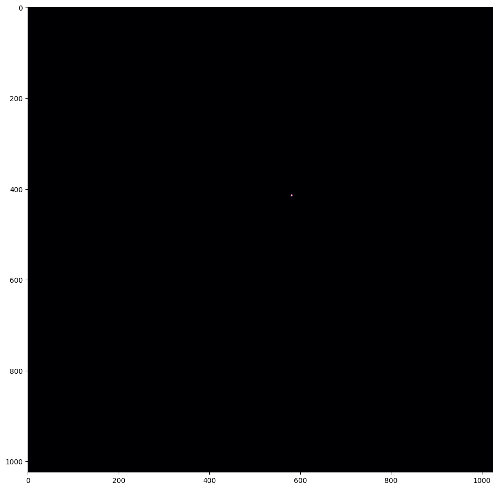
Great. Let’s take a look at the result in our camera with .get_image(). We’ll also set the exposure to an appropriate value; when running this notebook yourself, this might need to be adjusted.
[143]:
cam.set_exposure(29e-6)

img = cam.get_image()

assert np.max(img) > cam.bitresolution / 10, "The image is too dark. Try increasing the exposure time."

# Plot the result
plt.figure(figsize=(12,12))
plt.imshow(img)
plt.show()
We can also create a similar plot of the image with a simple call to .plot(), also taking advantage of the limits=.5 parameter to zoom in on the center 50% of the field of view:
[144]:
cam.plot(limits=.5, title="Image made with cam.plot()");
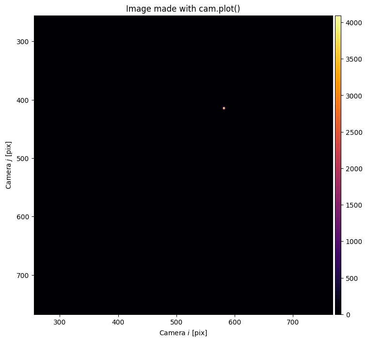
We see a spot corresponding to the zero-th order diffraction peak (i.e. undiffracted because no phase is written). This spot is focused near the center of our camera.
Next, we’ll move the laser spot by applying a blazed grating to the SLM using a helper function from our toolbox. This blazed grating has a Fourier spectrum shifted from the origin, so naturally applying this pattern to the SLM will produce a shifted result in the farfield, i.e. in the plane of the camera. Note that the phase pattern is in units of phase
(units of \(2\pi\)). This is then translated into the integer data that is actually displayed on the SLM (see .set_phase() or ._phase2gray()). If one passes integer phase to the SLM in .set_phase(), then this data is displayed directly, but any float data is interpreted as a phase. As an additional subtlety, most SLMs have an “increasing integer value, increasing voltage, decreasing phase” convention, so any passed phase is inverted in sign before displaying to have the
correct convention.
Many common phases patterns are available in the slmsuite.holography.toolbox.phase module, alongside blaze(). See the Structured Light Example for more information (e.g. the behavior of grid=).
We’re going to be .set_phase()ing .get_image()ing a couple more times in this notebook, so we’ll use the helper function fs.plot() to simplify plotting. One can also use cam.plot() and slm.plot() to plot the phase and amplitudes alone.
[145]:
from slmsuite.holography import toolbox

vector = (.002, .002)                                       # Radians (== normalized units kx/k).
blaze_phase = toolbox.phase.blaze(grid=slm, vector=vector)  # Phase in units of 2pi.

fs.plot(blaze_phase, title="blaze at {}".format(vector), cam_limits=.5);

Notice that the spot is now shifted. But what units does vector have? The default blaze units in slmsuite ("norm") are normalized \(k_x/k\) units, which are equivalent to radians in the small angle approximation. To get a better handle on what vector = (.002, .002) means, we can print the equivalent vectors
converted to supported units with toolbox.print_blaze_conversions() (n.b. "ij" is not yet calibrated so it cannot be converted).
[146]:
toolbox.print_blaze_conversions(vector=(.002, .002), from_units="norm", hardware=slm)
'rad' : [0.002 0.002]
'mrad' : [2. 2.]
'deg' : [0.11459156 0.11459156]
'norm' : [0.002 0.002]
'kxy' : [0.002 0.002]
'knm' : [739.10819672 435.40983607]
'freq' : [0.0442623 0.0442623]
'lpmm' : [4.09836066 4.09836066]
'zernike' : [166.98013929 166.98013929]
'ij' : [nan nan]
'm' : [nan nan]
'cm' : [nan nan]
'mm' : [nan nan]
'um' : [nan nan]
'nm' : [nan nan]
'mag_m' : [nan nan]
'mag_cm' : [nan nan]
'mag_mm' : [nan nan]
'mag_um' : [nan nan]
'mag_nm' : [nan nan]
C:\Users\holodyne\Documents\GitHub\slmsuite\slmsuite\holography\toolbox\__init__.py:258: UserWarning: CameraSLM must be passed as slm for conversion 'norm' to 'ij'
  warnings.warn(
C:\Users\holodyne\Documents\GitHub\slmsuite\slmsuite\holography\toolbox\__init__.py:258: UserWarning: CameraSLM must be passed as slm for conversion 'norm' to 'm'
  warnings.warn(
C:\Users\holodyne\Documents\GitHub\slmsuite\slmsuite\holography\toolbox\__init__.py:258: UserWarning: CameraSLM must be passed as slm for conversion 'norm' to 'cm'
  warnings.warn(
C:\Users\holodyne\Documents\GitHub\slmsuite\slmsuite\holography\toolbox\__init__.py:258: UserWarning: CameraSLM must be passed as slm for conversion 'norm' to 'mm'
  warnings.warn(
C:\Users\holodyne\Documents\GitHub\slmsuite\slmsuite\holography\toolbox\__init__.py:258: UserWarning: CameraSLM must be passed as slm for conversion 'norm' to 'um'
  warnings.warn(
C:\Users\holodyne\Documents\GitHub\slmsuite\slmsuite\holography\toolbox\__init__.py:258: UserWarning: CameraSLM must be passed as slm for conversion 'norm' to 'nm'
  warnings.warn(
C:\Users\holodyne\Documents\GitHub\slmsuite\slmsuite\holography\toolbox\__init__.py:258: UserWarning: CameraSLM must be passed as slm for conversion 'norm' to 'mag_m'
  warnings.warn(
C:\Users\holodyne\Documents\GitHub\slmsuite\slmsuite\holography\toolbox\__init__.py:258: UserWarning: CameraSLM must be passed as slm for conversion 'norm' to 'mag_cm'
  warnings.warn(
C:\Users\holodyne\Documents\GitHub\slmsuite\slmsuite\holography\toolbox\__init__.py:258: UserWarning: CameraSLM must be passed as slm for conversion 'norm' to 'mag_mm'
  warnings.warn(
C:\Users\holodyne\Documents\GitHub\slmsuite\slmsuite\holography\toolbox\__init__.py:258: UserWarning: CameraSLM must be passed as slm for conversion 'norm' to 'mag_um'
  warnings.warn(
C:\Users\holodyne\Documents\GitHub\slmsuite\slmsuite\holography\toolbox\__init__.py:258: UserWarning: CameraSLM must be passed as slm for conversion 'norm' to 'mag_nm'
  warnings.warn(
So we’re diffracting light by an angle of two milliradians or a tenth of a degree. You can read more about all the units in the documentation. Notice that some of the units are nan (and that we are warned about this). This is because we haven’t yet calibrated some needed conversions related to the relationship between the SLM’s
\(k\)-space and the camera’s pixel space, but more on that next section.
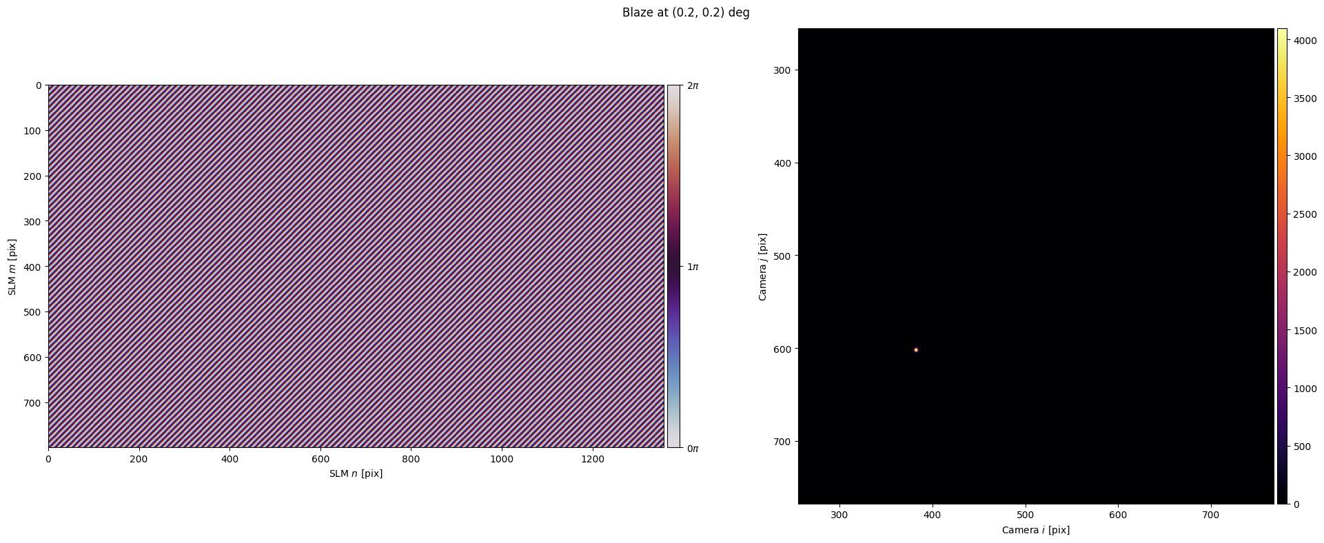
This function wraps toolbox.convert_vector() which handles arbitrary unit conversions. Let’s try it out by diffracting light at .2 degrees in the \(x\) and \(y\) directions.
[147]:
# Get .2 degrees in normalized units.
vector_deg = (.2, .2)
vector = toolbox.convert_vector(vector_deg, from_units="deg", to_units="norm")

# Get the phase for the new vector
blaze_phase = toolbox.phase.blaze(grid=slm, vector=vector)

fs.plot(blaze_phase, title="Blaze at {} deg".format(vector_deg), cam_limits=.5);
All this is good fun, but let’s say we wanted our spot right at pixel (500, 700). We could iterate by guessing and checking successive vectors, but that seems boring and non-pythonic. Instead, we will calibrate a transformation between the \(k\)-space of the SLM and the space of the camera using features built-in to slmsuite.
Fourier Calibration#
Calibration is simple, just run a built-in function .fourier_calibrate() to 1) generate and 2) fit a grid of spots (with known \(k\)-space coordinates) with an affine transformation to the space of the camera. This grid is generated using the same holography algorithms we explored in the computational holography tutorial. We’ll come back to experimental implementations of these shortly; for now, care
must be taken to choose:
A camera exposure such that spots are prominent,
A pitch and shape of the array which are visually resolvable.
Note that the default array units are in "knm" space, or the computational space of holography. Read more about this in later examples.
[148]:
cam.set_exposure(5e-4)              # Increase exposure because power will be split many ways

fs.fourier_calibrate(
    array_shape=20,                 # Size of the calibration grid (Nx, Ny) [#]
    array_pitch=20,                 # Pitch of the calibration grid (x, y) [knm]
    plot=True
);
C:\Users\holodyne\Documents\GitHub\slmsuite\slmsuite\holography\toolbox\__init__.py:258: UserWarning: CameraSLM must be passed as slm for conversion 'kxy' to 'ij'
  warnings.warn(
Notice that there are two missing spots from the array. This is a parity check to make sure the calibration is flipped in the correct direction.
The result of this process is the transformation
\(\vec{x} = M \cdot (\vec{k} - \vec{a}) + \vec{b}\)
where \(\vec{x}\) is in units of camera pixels and \(\vec{k}\) is in units of normalized \(k\)-space. We can view the result in the fourier_calibration variable.
[149]:
fs.calibrations["fourier"]
[149]:
{'M': array([[-56019.5350493 ,   -927.92347037],
        [  -947.50892215,  54745.58678092]]),
 'b': array([[581.86927324],
        [414.82425824]]),
 'a': array([[ 8.76122968e-21],
        [-1.40179675e-19]]),
 '__version__': '0.4.0',
 '__time__': '2026-03-22 15:02:57.723188',
 '__timestamp__': 1774206177.723188,
 '__meta__': {'__class__': '<slmsuite.hardware.cameraslms.FourierSLM object at 0x00000265C03BBFD0>',
  'name': '22562470-p67',
  'cam': {'__class__': '<slmsuite.hardware.cameras.flir.FLIR object at 0x00000265C03BAB30>',
   'name': '22562470',
   'shape': (1024, 1024),
   'bitdepth': 12,
   'bitresolution': 4096,
   'pitch_um': array([2.74, 2.74]),
   'exposure_s': 0.0005,
   'exposure_bounds_s': (2.9e-05, 30.00001),
   'averaging': None,
   'hdr': None,
   'woi': (2148, 1024, 1000, 1024),
   'default_shape': (3032, 5320)},
  'slm': {'__class__': '<slmsuite.hardware.slms.texasinstruments.PLM object at 0x00000265B8430E50>',
   'name': 'p67',
   'shape': (800, 1358),
   'bitdepth': 4,
   'bitresolution': 16,
   'pitch_um': array([10.8, 10.8]),
   'pitch': array([22.13114754, 22.13114754]),
   'settle_time_s': 0.05,
   'wav_um': 0.488,
   'wav_design_um': 0.488,
   'phase_scaling': 1.0},
  'mag': 1.0}}
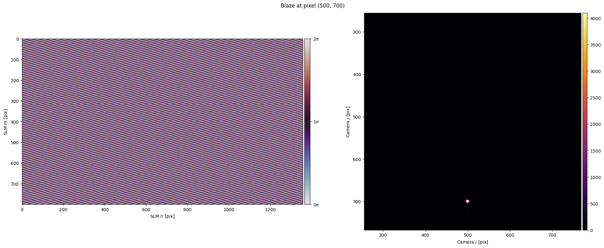
Now let’s use this calibration to achieve our goal of (500, 700). We can find the blaze vector \(\vec{k}\) (in normalized units) corresponding to the desired pixel \(\vec{x}\) using our calibration.
[150]:
vector_500_700 = fs.ijcam_to_kxyslm((500, 700))
print(vector_500_700)
[[0.00137476]
 [0.0052329 ]]
Now let’s check this result:
[151]:
blaze_phase = toolbox.phase.blaze(grid=slm, vector=vector_500_700)

fs.plot(blaze_phase, title="Blaze at pixel (500, 700)", cam_limits=.5)

cam.set_exposure(29e-6)
img = cam.get_image()
assert np.mean(img[690:710, 490:510]) > np.mean(img), "Make sure most of the power is in the expected area."
Let’s also go back to print_blaze_conversions. With the extra information from Fourier calibration stored in fs (now passed as hardware=), all the units are now filled out.
[152]:
toolbox.print_blaze_conversions(vector=vector_500_700, from_units="norm", hardware=fs)
'rad' : [0.00137476 0.0052329 ]
'mrad' : [1.37476221 5.23290293]
'deg' : [0.07876807 0.29982325]
'norm' : [0.00137476 0.0052329 ]
'kxy' : [0.00137476 0.0052329 ]
'knm' : [720.31723867 492.64811737]
'freq' : [0.03042507 0.11581015]
'lpmm' : [ 2.81713568 10.72316173]
'zernike' : [114.77899264 436.89542969]
'ij' : [500. 700.]
'm' : [0.00137  0.001918]
'cm' : [0.137  0.1918]
'mm' : [1.37  1.918]
'um' : [1370. 1918.]
'nm' : [1370000. 1918000.]
'mag_m' : [0.00137  0.001918]
'mag_cm' : [0.137  0.1918]
'mag_mm' : [1.37  1.918]
'mag_um' : [1370. 1918.]
'mag_nm' : [1370000. 1918000.]
Spot Holography#
The previous examples considered blazing light in one direction towards one point, but what if we want to generate patterns with many spots? Of course, this isn’t as simple as adding the blaze phase patterns for \(\vec{k}_1\) and \(\vec{k}_2\), as this would just blaze light along \(\vec{k} = \vec{k}_1 + \vec{k}_2\). Things are more complicated. This example will show how to generate SpotHolograms with slmsuite.
A Square Array and take#
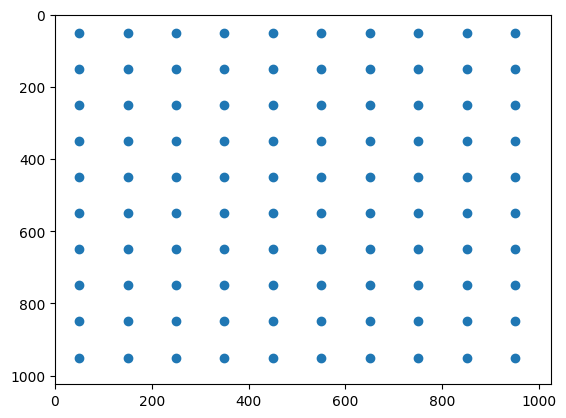
Let’s consider a case where we want to fill part of our camera’s space with a square array of spots, spaced with a pitch of 100 pixels.
[153]:
xlist = np.arange(50, min(fs.cam.shape)-50, 100)                      # Get the coordinates for one edge
print(xlist)

xgrid, ygrid = np.meshgrid(xlist, xlist)
square = np.vstack((xgrid.ravel(), ygrid.ravel()))                  # Make an array of points in a grid

plt.scatter(square[0,:], square[1,:])                               # Plot the points
plt.xlim([0, fs.cam.shape[1]]); plt.ylim([fs.cam.shape[0], 0])
plt.show()
[ 50 150 250 350 450 550 650 750 850 950]
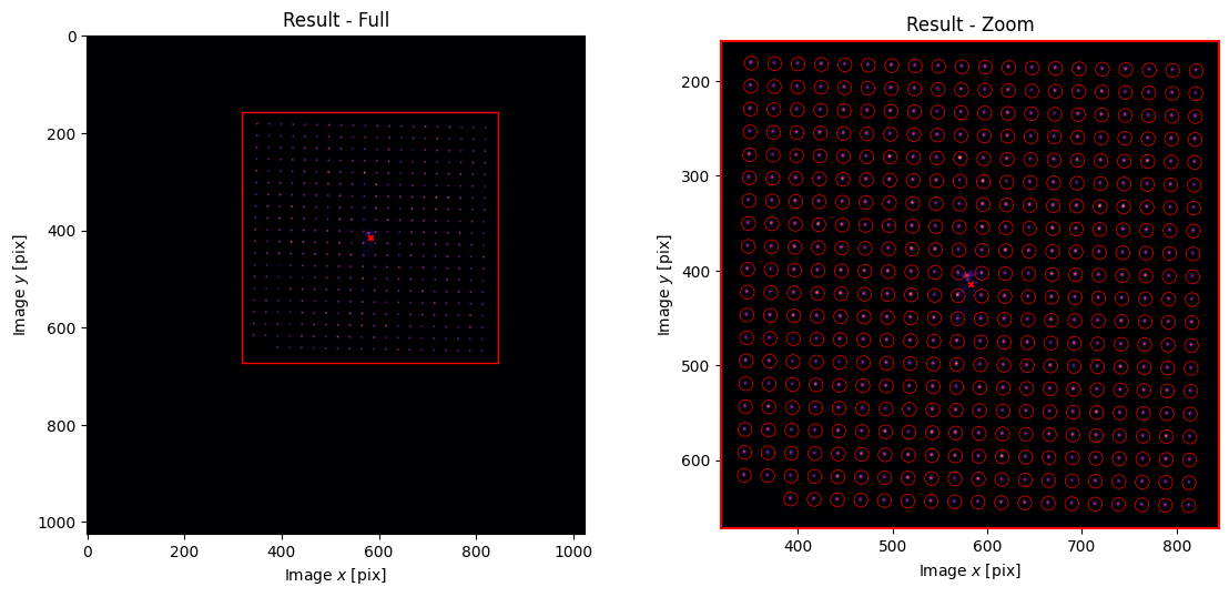
Making a hologram is simple. we initialize a hologram with a computational space of shape (2048, 2048). This shape just has to be larger than the SLM shape, and should ideally consist of powers of two. We provide the points in the "ij" basis of our camera’s pixels, made possible by the Fourier calibration passed via our FourierSLM named fs.
[154]:
from slmsuite.holography.algorithms import SpotHologram
hologram = SpotHologram(shape=(2048, 2048), spot_vectors=square, basis='ij', cameraslm=fs)
This initialize just constructs datastructures, but does not conduct optimization.
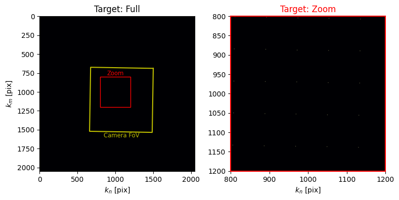
We can first plot the target amplitudes at desired locations in the "knm" basis, which is needed to apply discrete Fourier transforms. Our Fourier calibration also shows us how our camera’s field of view (in yellow) compares to the size of the computational space.
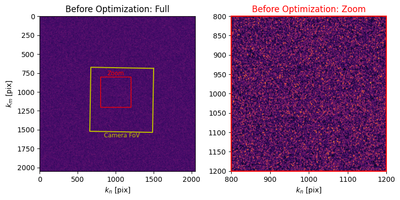
Next, we plot the amplitudes resulting from the initial conditions of optimization (random phase). This just looks like noise, as expected.
[155]:
hologram.plot_farfield(hologram.target,  limits=[[800, 1200], [800, 1200]], title="Target")
hologram.plot_farfield(limits=[[800, 1200], [800, 1200]], title="Before Optimization");
This randomness won’t last. We quickly take 50 iterations of optimization towards our target. Here, we use weighted Gerchberg-Saxton-type algorithms to iteratively hone the nearfield phase pattern to produce the desired farfield at the camera.
[156]:
cam.set_exposure(.002)              # Increase exposure because power will be split many ways
hologram.optimize('WGS-Kim', feedback='computational_spot', stat_groups=['computational_spot'], maxiter=50)
hologram.plot_farfield(limits=[[800, 1200], [800, 1200]], title="After Optimization");
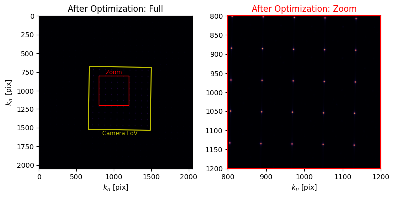
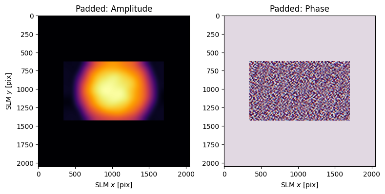
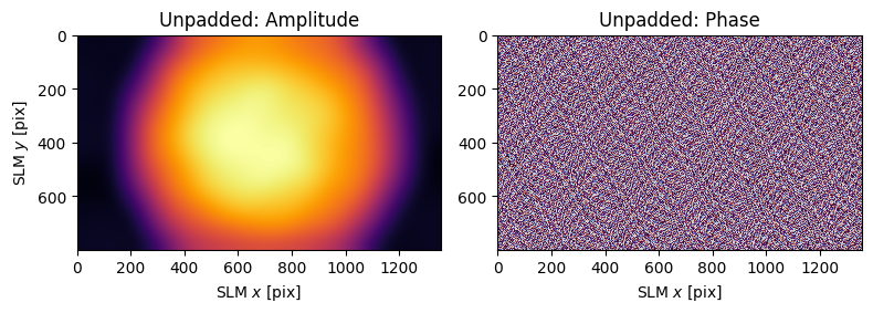
Now the computed result of our optimized hologram roughly matches the target. The phase that generates this amplitude result in the farfield is plotted below. The amplitude pattern is an estimate of the real nearfield amplitude measured via wavefront calibration. Note that we plot both the system padded to the (2048, 2048) shape of the computational space (used during optimization) and the system cropped to the shape of the SLM (used in practice).
[157]:
hologram.plot_nearfield(title="Padded", padded=True)
hologram.plot_nearfield(title="Unpadded")
Let’s see how this looks experimentally.
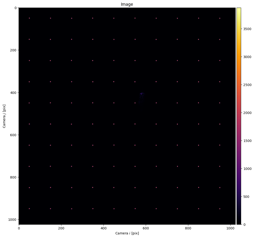
[158]:
fs.slm.set_phase(hologram.get_phase(), settle=True)                 # Write hologram.
fs.cam.flush()
img = fs.cam.get_image()                                        # Grab image.

plt.figure(figsize=(12,12))
fs.cam.plot(img);

Looks good! Those two extra spots below the zero-th order are due to reflections off of the 50:50 beamsplitter. A setup without a beamsplitter would not have these artifacts.
We can immediately see (even through the saturation) that the spots on the edges of the field of view are less bright. Let’s take() a closer look at this making using of helper functions in the analysis module. The function take() is very useful to analyze spots. It crops an image into many windows with width size around a desired set of vector, in our case, the points at which we expects spots to appear. take() is written to be efficient, making heavy use of numpy
parallelism, and has many useful options.
We also plot the regions we took from the image using the take_plot() helper function.
[159]:
from slmsuite.holography import analysis

subimages = analysis.take(img, vectors=square, size=15)
assert np.mean(subimages) > np.mean(img) / 2, "Make sure the subimages cover most of the power in the image."

analysis.take_plot(subimages, separate_axes=True)

The spots are a pixel off in a few places, but a bigger issue is the uniformity. We can get a histogram of the spot powers with another helper function image_normalization().
[160]:
powers = analysis.image_normalization(subimages)

powers_norm = powers / np.mean(powers)
powers_norm_std_gs = np.std(powers_norm)

plt.hist(powers_norm)
plt.title("GS Powers (std={:.2f}%)".format(powers_norm_std_gs * 100))
plt.show()
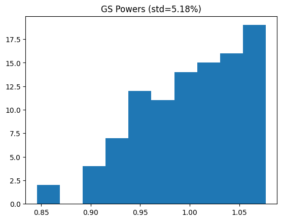
There’s a good amount of variation across the array, some might result from diffraction inefficiency closer to the field of view. In practice, the closer to the edge of the \(k\)-space one gets, the lower the efficiency due to sampling considerations. A solution lies in camera feedback, a focus of slmsuite as a package that considers the unification of SLMs and cameras.
A Uniform Square Array#
We can easily enable camera feedback by using the option to feedback upon the power at spots measured by the camera. This is enabled by switching to "experimental_spot" (versus "computational_spot") feedback. Since the optimization with experimental feedback is a bit slower (we wait for the SLM to settle and for the camera to grab an image), we precondition our optimization computationally-optimized pattern.
[161]:
hologram = SpotHologram(shape=(2048, 2048), spot_vectors=square, basis='ij', cameraslm=fs)

# Precondition computationally.
hologram.optimize(
    'WGS-Kim',
    maxiter=20,
    feedback='computational_spot',
    stat_groups=['computational_spot']
)
# Hone the result with experimental feedback.
hologram.spot_integration_width_ij = 15
hologram.optimize(
    'WGS-Kim',
    maxiter=20,
    feedback='experimental_spot',
    stat_groups=['computational_spot', 'experimental_spot'],
    fixed_phase=False
)
And let’s take a look at our result.
[162]:
# Grab image (this time we dont' have to .set_phase() to the SLM, because the
# optimization did this already).
img = fs.cam.get_image()

plt.figure(figsize=(12,12))
fs.cam.plot(img);
This looks more uniform, but it’s hard to tell from the saturation. Let’s take another look at the statistics of our array.
[163]:
subimages = analysis.take(img, vectors=square, size=hologram.spot_integration_width_ij)
powers = analysis.image_normalization(subimages)

powers_norm = powers / np.mean(powers)
powers_norm_std_wgs = np.std(powers_norm)

assert powers_norm_std_wgs < powers_norm_std_gs, "Make sure that the distribution got more uniform."

plt.hist(powers_norm)
plt.title("WGS Powers (std={:.2f}%)".format(powers_norm_std_wgs * 100))
plt.show()
Much more uniform. With the stat_groups parameter, we also asked the SpotHologram to note statistics as the optimization proceeded. We can plot these with the .plot_stats() function.
[164]:
hologram.plot_stats();
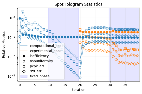
This begs the question of what limits uniformity. In the case of this setup, it’s likely the precision of our camera and the fact that power is concentrated on only a few of these 8-bit pixels.
A Scattered Example#
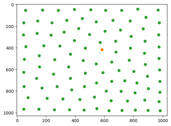
Lloyd’s Algorithm iteratively generates an array of spots spread across a given space. In this case, we want to generate a cloud of points within the field of view of our camera.
[165]:
lloyds_points = toolbox.lloyds_points(grid=fs.cam.shape, n_points=100, iterations=40)
Let’s remove the point closest to the zeroth order and then take a look at what we generated.
[166]:
zeroth_order_ij = fs.kxyslm_to_ijcam((0,0))

plt.scatter(lloyds_points[0, :], lloyds_points[1, :], alpha=.1)
plt.scatter(zeroth_order_ij[0], zeroth_order_ij[1])
difference_vectors = lloyds_points - zeroth_order_ij
distance_to_zeroth = np.sqrt(np.square(difference_vectors[0, :]) + np.square(difference_vectors[1, :]))
closest_to_zeroth = np.argmin(distance_to_zeroth)
lloyds_points = np.delete(lloyds_points, closest_to_zeroth, 1)
plt.scatter(lloyds_points[0, :], lloyds_points[1, :])
plt.gca().set_ylim(np.flip(plt.gca().get_ylim()))
plt.show()
We conduct the same process to optimize a hologram to generate this pattern.
[167]:
hologram = SpotHologram((2048, 2048), lloyds_points, basis='ij', cameraslm=fs)

# Precondition computationally.
hologram.optimize(
    'WGS-Kim',
    maxiter=20,
    feedback='computational_spot',
    stat_groups=['computational_spot']
)
# Hone the result with experimental feedback.
hologram.optimize(
    'WGS-Kim',
    maxiter=20,
    feedback='experimental_spot',
    stat_groups=['computational_spot', 'experimental_spot'],
    fixed_phase=False
)
Let’s again take a look at what we generated.
[168]:
img = fs.cam.get_image()

plt.figure(figsize=(24,24))
ax = fs.cam.plot(img)
ax.scatter(lloyds_points[0, :], lloyds_points[1, :], 1600, facecolors='none', edgecolors='r')
plt.show()
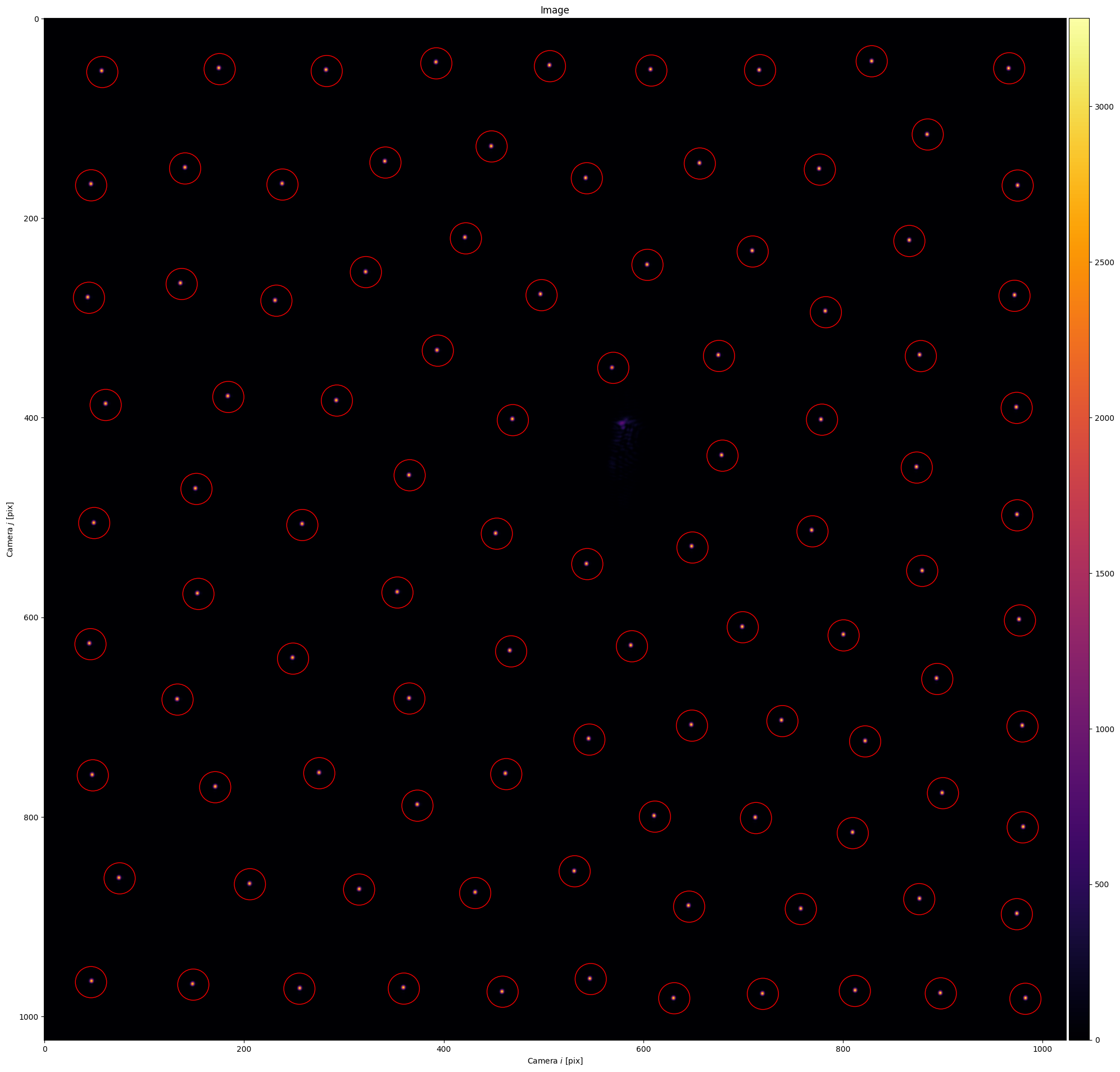
Let’s again take a look at the statistics. The optimization was faster, as expected for a pattern with less crystallinity.
[169]:
hologram.plot_stats();

Pictorial Holography#
The spot holography we explored above is a subset of the general problem. In this section, we push further and look into forming images at desired positions in the camera’s domain.
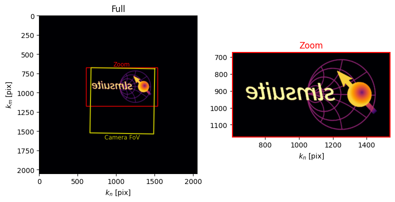
Let’s start by loading a picture. We load an example helper function for this.
[170]:
from slmsuite.holography.analysis.files import _load_image
path = os.path.join(os.getcwd(), '../../slmsuite/docs/source/static/slmsuite-small.png')
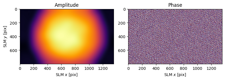
target_ij = _load_image(path, fs.cam.shape, angle=0, shift=(-225, 0))
plt.figure(figsize=(16,12))
fs.cam.plot(target_ij)
plt.plot(target_ij.shape[1]/2, target_ij.shape[0]/2, 'r*');

Notice that the resulting image has the same shape as the camera. The goal is to replicate this pattern on the camera at the same position. We use similar syntax as before to initialize and optimize the hologram. This time we use a FeedbackHologram, which is actually the superclass of SpotHologram. FeedbackHologram is a subclass of Hologram, a class that only considers the abstract. FeedbackHologram has infrastructure to read in and interpret camera images. SpotHologram
has infrastructure honed to optimize spot arrays. Let’s take a look at our FeedbackHologram.
[171]:
from slmsuite.holography.algorithms import FeedbackHologram
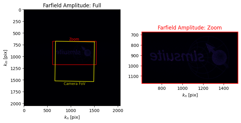
hologram = FeedbackHologram(shape=(2048, 2048), target_ij=target_ij, cameraslm=fs);
limits = hologram.plot_farfield(hologram.target);
hologram.reset_phase(quadratic_phase=2)
We see how the image is imprinted upon the "knm" space in which the hologram is optimized. Now let’s optimize it.
[172]:
hologram.optimize(
    method="WGS-Leonardo",
    maxiter=10,
    feedback='computational',
    stat_groups=['computational']
)
We quickly plot the image, and see our hologram! It looks alright.
[173]:
cam.set_exposure(.1)

slm.set_phase(hologram.get_phase(), settle=True)

plt.figure(figsize=(12,12))
cam.plot();

This is the phase that produces that result.
[174]:
hologram.plot_nearfield()
We can also take a look at the hologram computationally, i.e. the expected result from Fourier-transforming the nearfield. Notice that there is some power in the field, and we need to use the limits from the previous .plot_farfield() to get the zoom box to not be the whole domain.
[175]:
hologram.plot_farfield(limits=limits);
We can push this a bit further by again applying camera feedback, this time to the whole image.
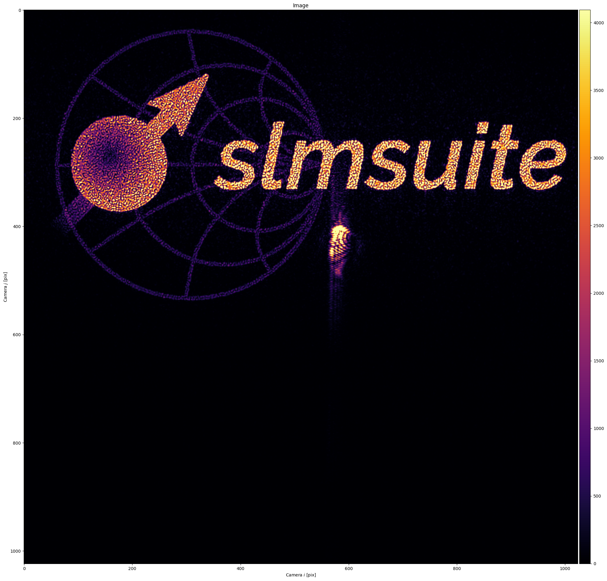
[176]:
hologram.optimize(
    method="WGS-Leonardo",
    maxiter=10,
    feedback='experimental',
    stat_groups=['computational', 'experimental'],
    blur_ij=1
)
The hologram appears with higher fidelity, though speckle remains a concern.
[177]:
slm.set_phase(hologram.get_phase(), settle=True)

plt.figure(figsize=(24,24))
cam.plot();
We look forward to seeing what sort of holograms you’ll make!
[178]:
cam.close()
slm.close()