

Structured Light#
This example discusses helper functions and details for manipulating phase patterns: mainly regarding the contents of slmsuite.holography.toolbox.phase.
Initialization#
This tutorial can be run optionally with or without hardware connected. The below code block tries to load physical hardware and cleanly falls back to virtual hardware if loading fails. We also try to load the wavefront calibration from a previous tutorial.
[2]:
# Try to load physical hardware.
try:
from slmsuite.hardware.slms.texasinstruments import PLM
from slmsuite.hardware.cameras.flir import FLIR
# Load the hardware.
slm = PLM('p67', 1, wav_um=0.488, settle_time_s=0.05, configure_usb=True); print()
cam = FLIR(serial="22562470", pitch_um=2.74)
# For this camera, we also want to crop the WOI to the center 1024x1024 area.
h_max, w_max = cam.default_shape
cam.set_woi(((w_max - 1024) // 2, 1024, (h_max - 1024) // 2, 1024))
# Load the composite CameraSLM.
fs = FourierSLM(cam, slm)
fs.load_calibration("wavefront_superpixel"); # We'll come back to this next tutorial!
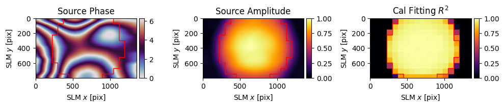
fs.wavefront_calibration_superpixel_process(plot=True, r2_threshold=.8)
# Fallback to virtual hardware.
except Exception as e:
print(f"Loading physical hardware failed; loading virtual hardware. Error:\n{str(e)}")
from slmsuite.hardware.slms.simulated import SimulatedSLM
from slmsuite.hardware.cameras.simulated import SimulatedCamera
# Make the SLM and camera.
slm = SimulatedSLM((1600, 1200), pitch_um=(8,8))
# Program the simulated and calibrated sources to be flat phase.
slm.set_source_analytic(sim=True)
slm.set_source_analytic()
cam = SimulatedCamera(slm, (1440, 1100), pitch_um=(4,4), gain=200)
# Tie the camera and SLM together with an analytic calibration.
fs = FourierSLM(cam, slm)
M, b = fs.fourier_calibration_build(
f_eff=80000., # f_eff of 80000 wavelengths or 80 mm with the default 1 um wavelength
theta=5 * np.pi / 180,
)
cam.set_affine(M, b)
fs.fourier_calibrate_analytic(M, b)
PLM using GPU (cupy) backend
DLPC900 connected: firmware {'app_version': 95, 'api_version': 72, 'sw_patch': 111, 'sw_minor': 108, 'sw_major': 111}
DLPC900 pre-configured (video mode, display detected)
Initializing pyglet... success
Searching for window with display_number=1... success
Creating window... Window creation successful
DLPC900 source locked, switching to video-pattern mode...
DLPC900 configured successfully - pattern sequence running

PySpin initializing... Looking for cameras... PySpin sn '22562470' initializing... PixelFormat set to Mono16 (12-bit)... Frame rate set to 33.7 Hz... Successfully initialized FLIR cam 22562470.
C:\Users\holodyne\Documents\GitHub\slmsuite\slmsuite\hardware\cameraslms.py:3720: UserWarning: remove_background is enabled and a noise floor was detected; removing this background (0.06709127128124237% of the average normalization).
  warnings.warn(
When running on physical hardware, you’ll need to set the exposure of the camera to get appropriate results (the exposure setting in this notebook is mostly overexposed for generality, but isn’t necessarily ideal for all examples).
[3]:
cam.set_exposure(.0001);
Simple Blazes & Lenses#
Linear phase ramps, also known as blazes after blazed gratings, are a useful analytic function for SLM usage. In this package, slmsuite.holography.toolbox.phase.blaze implements this function. We can compute the blaze towards the direction of vector. This vector is in normalized \(\frac{k_x}{k}\) units (see slmsuite.holography.toolbox.convert_blaze_vector for more information and unit conversions), and the x_grid and y_grid coordinates are likewise interpreted to be
normalized to wavelength.
[4]:
from slmsuite.holography import toolbox
from slmsuite.holography.toolbox import phase

x_list = np.arange(2000)
y_list = np.arange(1000)
x_grid, y_grid = np.meshgrid(x_list, y_list)

blaze_phase = phase.blaze(
    grid=(x_grid, y_grid),          # Coordinates of our SLM pixels.
    vector=(.002, .002)             # Angle vector (in normalized units) to blaze towards.
)
Then, we can render our result using matplotlib, with the aid of a quick helper function plot() which is present in each Camera, SLM, and CameraSLM:
[5]:
fs.slm.plot(blaze_phase, title="blaze_phase");

However, making and tracking x_grid and y_grid is an unwieldy pain. We encourage users to not do this unless necessary and instead use convenience features builtin to blaze and similar toolbox functions. For instance, we can pass an SLM directly in place of the grids:
[6]:
blaze_phase_easy = phase.blaze(
    grid=slm,                       # Coordinates of our SLM pixels, inherited from the SLM.
    vector=(.002, .002)             # Again, angle vector (in normalized units) to blaze towards.
)

# Plotting.
fs.plot(blaze_phase_easy, title="blaze_phase_easy", cam_limits=.5);
plt.show()

no_blaze = phase.blaze(grid=slm, vector=(0,0))
fs.plot(no_blaze, title="no_blaze", cam_limits=.5);


At startup, the SLM caches grids with appropriate shape and dimension, using the coordinates normalized to the target wavelength \((\frac{x}{\lambda}, \frac{y}{\lambda})\) which blaze expects. These grids are stored in slm.x_grid and slm.x_grid, and passing grid=slm is equivalent to passing grid=(slm.x_grid, slm.y_grid).
Note that these grids are centered on the SLM, such that when we try other helper functions such as slmsuite.holography.toolbox.phase.lens, the result is centered:
[7]:
lens_phase = phase.lens(
    grid=slm,
    f=1e7                       # Focal length in wavelengths.
)

fs.plot(lens_phase, title="lens_phase", cam_limits=.5);

As before, units are normalized to wavelength, so passing f=1e7 is equivalent to requesting a lens with a focal length of ten million wavelengths, or 6.33 meters at 633 nm.
We can of course pass more interesting lenses. For instance, an elliptical lens:
[8]:
elliptical_phase = phase.lens(
    grid=slm,
    f=(2e7, 1e7)                # Focal length in the x and y directions.
)

fs.plot(elliptical_phase, title="elliptical_phase", cam_limits=.5);

Or going further to a cylindrical lens:
[9]:
cylindrical_phase = phase.lens(
    grid=slm,
    f=(np.inf, 1e7)             # x direction is now unfocused.
)

fs.plot(cylindrical_phase, title="cylindrical_phase", cam_limits=.5);

Pattern Basis Transformations#
The patterns we looked at thus far have been all centered at the origin. We can use toolbox.shift_grid()
Or rotate the lens about the center:
[10]:
rotated_phase = phase.lens(
    grid=toolbox.transform_grid(
        slm,
        transform=np.pi/4,                  # Angle in radians to rotate by.
        shift=(0, 0)
    ),
    f=(2e7, 1e7)
)

fs.plot(rotated_phase, title="rotated_phase", cam_limits=.5);

Or shift the center across the SLM. Note that center, like other parameters in slmsuite, is in normalized units. Fortunately, the slm has helper variables dx and dy which store the pixel size in normalized units, such that requesting a (800, -400) pixel shift is as simple as multiplying by these variables to convert to normalized units:
[11]:
shifted_phase = phase.lens(
    grid=toolbox.transform_grid(
        slm,
        transform=np.pi/4,
        shift=(800*slm.pitch[0], -400*slm.pitch[1])     # Shift of the center of the SLM.
    ),
    f=(2e7, 1e7)
)

fs.plot(shifted_phase, title="shifted_phase", cam_limits=.5);

We can see a slight shift from the zero-th order, the expected result from the amount of linear blaze that is equivalent to shifting the quadratic lens on the SLM.
Structured Light Conversion#
There are a number interesting optical modes whose farfield pattern is Gaussian in amplitude, with the addition of some phase. As the beam sourced on an SLM is often in a Gaussian mode, we can tune phase on the SLM to produce structured light in the nearfield of the camera. One example is a Laguerre-Gaussian mode, possessing the optical analog of orbital angular momentum. To start, we can take a look at the phase for a \(LG_{lp} = LG_{10}\) mode, also known as a vortex waveplate (this pattern is hard to see on the camera because the resulting ring pattern is small and overexposed):
[12]:
lg10_phase = phase.laguerre_gaussian(
    slm,
    l=1,                                        # Azimuthal wavenumber
    p=0                                         # Radial wavenumber
)

fs.plot(lg10_phase, title="lg10_phase", cam_limits=.5);

Higher order vortex phases such as for a \(LG_{lp} = LG_{90}\) mode are easy to see on the camera:
[13]:
lg90_phase = phase.laguerre_gaussian(
    slm,
    l=9,                                        # A larger azimuthal wavenumber
    p=0
)

fs.plot(lg90_phase, title="lg90_phase", cam_limits=.5);

The asymmetry of the resulting mode is likely due to imperfect centering of the incident beam on the SLM. Higher order and more interesting modes are also possible, such as for a \(LG_{lp} = LG_{93}\) mode:
[14]:
lg93_phase = phase.laguerre_gaussian(
    slm,
    l=9,
    p=3                                         # Nonzero radial wavenumber
)

fs.plot(lg93_phase, title="lg93_phase", cam_limits=.5);

We can do cool things like shift the beam by adding a blaze.
[15]:
lg93_shifted_phase = lg93_phase + phase.blaze(grid=slm, vector=(.002, .002))

fs.plot(lg93_shifted_phase, title="lg93_shifted_phase", cam_limits=.5);

Or we can defocus the beam by adding a lens.
[16]:
lg93_defocused_phase = lg93_phase + phase.lens(grid=slm, f=1e7)

fs.plot(lg93_defocused_phase, title="lg93_defocused_phase", cam_limits=.5);

We also implement Hermite-Gaussian conversion. Shown below is the phase for a \(HG_{nm} = HG_{11}\) mode:
[17]:
hg11_phase = phase.hermite_gaussian(
    grid=slm,
    n=1,                                        # x wavenumber
    m=1                                         # y wavenumber
)

fs.plot(hg11_phase, title="hg11_phase", cam_limits=.5);

Although we admittedly haven’t gotten around to implementing these yet, there are also ince_gaussian and matheui_gaussian beam conversions planned for toolbox. We welcome contributions if you want to finish these!
Segmented SLMs and imprint#
In some cases, it is desirable to split an SLM into many individual regions. slmsuite has helper functions to support this.
The slmsuite.toolbox.imprint() operation ‘imprints’ a function such as blaze and lens from the previous section onto the SLM, but only in a given window. This window can be defined many ways (see API reference), but here we define it in (x, w, y, h) form. Extra keyword arguments to imprint are passed to the function. This function is used, for instance, to make the superpixels used for wavefront calibration. See the below examples for three superpixels producing three offset
first order diffraction peaks, while most of the field and the zeroth order remain centered.
[24]:
# Setup some parameters for a grid of imprinted blazes.
dk = .001
size = 400
cx1, cy1 = np.flip(slm.shape) // 2
cx0 = cx1 - size
cy0 = cy1 - size

# Setup a blank canvas
canvas = np.zeros(shape=slm.shape)

# Imprint three windows, with different blazes.
toolbox.imprint(canvas, window=[cx0, size, cy0, size], function=phase.blaze, grid=slm, vector=( dk,  dk))
toolbox.imprint(canvas, window=[cx1, size, cy0, size], function=phase.blaze, grid=slm, vector=(-dk,  dk))
toolbox.imprint(canvas, window=[cx0, size, cy1, size], function=phase.blaze, grid=slm, vector=(-dk, -dk))
toolbox.imprint(canvas, window=[cx1, size, cy1, size], function=phase.blaze, grid=slm, vector=(-dk, 0))

fs.plot(canvas, title="imprint_canvas", cam_limits=.5);

imprint() supports two operation types:
imprint_operation="replace", the default, where the original phase on thecanvasis overwritten, andimprint_operation="add", where the original phase is instead added to.
In the example below, phase in the middle window is zeroed, as the field had the negative of the imprinted phase. The right box adds to create a new vector.
[25]:
# Use a non-zero base canvas to help explain available operations.
canvas = phase.blaze(grid=slm, vector=(dk, -dk))

# Imprint three windows, now with different operations.
toolbox.imprint(canvas, window=[cx0, size, cy0, size], function=phase.blaze, grid=slm, vector=( dk,  dk), imprint_operation="replace")
toolbox.imprint(canvas, window=[cx1, size, cy0, size], function=phase.blaze, grid=slm, vector=(-dk,  dk), imprint_operation="add")
toolbox.imprint(canvas, window=[cx0, size, cy1, size], function=phase.blaze, grid=slm, vector=(-dk, -dk), imprint_operation="add")
toolbox.imprint(canvas, window=[cx1, size, cy1, size], function=phase.blaze, grid=slm, vector=(-dk, 0),   imprint_operation="add")

fs.plot(canvas, title="operation_canvas", cam_limits=.5);

Now suppose we want to something more complicated, with very many regions on the same SLM instead of a handful. As an example, we can make an array of microlenses on a grid. First of all, we have helper functions to construct the grid. The function toolbox.fit_3pt() can construct an affine transformation based on three given vectors (y0, y1, y2), and return a grid of vectors with size N:
[26]:
vectors = toolbox.fit_3pt(y0=(200,100), y1=(300,110), y2=(220, 200), N=(10,6))
This is only a fraction of what toolbox.fit_3pt() can do; see the API reference for the full capabilities of this function. We can quickly visualize this to see we indeed have a grid:
[27]:
plt.figure(figsize=(10,5))
plt.plot(vectors[0,:], vectors[1,:], "*")       # Plot the points at which cells are desired.
plt.xlim(0, slm.shape[1])
plt.ylim(slm.shape[0], 0)
plt.gca().set_aspect('equal')
plt.show()

Now we can use imprint to add a lens at each point. For now we’ll use a width and height of width = 50 pixels. We’re also using the centered parameter of imprint such that the vector position of the window is centered instead of at the lower left corner.
[28]:
slm.source.keys()
[28]:
dict_keys(['phase', 'amplitude', 'r2', 'r2_threshold', 'amplitude_center_pix', 'amplitude_radius', 'amplitude_extent', 'amplitude_extent_radius'])
[29]:
width = 50

def get_segmented_phase_square(width):
    N = vectors.shape[1]
    segmented_phase_square = np.zeros(shape=slm.shape)

    for x in range(N):
        vector_normalized = (
            -(vectors[0,x] - slm.source["amplitude_center_pix"][0]) * slm.pitch[0],
            -(vectors[1,x] - slm.source["amplitude_center_pix"][1]) * slm.pitch[1]
        )
        # Imprint a lens in a square window about each point.
        toolbox.imprint(
            segmented_phase_square,
            window=[vectors[0,x], width, vectors[1,x], width],
            function=phase.lens,
            grid=slm,
            f=np.random.uniform(5e4, 1e5),
            shift=vector_normalized,
            centered=True
        )

    return segmented_phase_square

fs.slm.plot(get_segmented_phase_square(width), title="segmented_phase_square");

This is interesting, but we should try for better fill factor. We can use another helper function toolbox.get_smallest_distance() and the Chebyshev metric \(\max_i|u_i - v_i|\) to find the largest window size that doesn’t collide with other boxes.
[30]:
import scipy.spatial.distance as distance

# Find the maximum width that avoids overlapping windows.
width = toolbox.smallest_distance(vectors, metric=distance.chebyshev)
print("Max width: ", width)

fs.slm.plot(get_segmented_phase_square(width), title="segmented_phase_square_larger");
Max width: 90.0

Better, but there’s still some empty space that we might want to fill. The helper function toolbox.get_voronoi_windows can help with this, making a Voronoi cell around each point.
[31]:
windows = toolbox.voronoi_windows(
    grid=slm.shape,                     # Shape of the canvas of returned boolean windows.
    vectors=vectors,                    # Points to make Voronoi cells around.
    plot=True
)

This function returns a list of windows, where each window is a boolean array.
[32]:
plt.figure(figsize=(10,5))
plt.imshow(windows[21])         # Plot the 21st window.
plt.show()

Such windows can be passed to imprint, where the function will only be evaluated and imprinted within the defined area.
[33]:
def get_segmented_phase(windows):
    N = vectors.shape[1]
    segmented_phase = np.zeros(shape=slm.shape)

    for x in range(N):
        vector_normalized = (
            -(vectors[0,x] - slm.source["amplitude_center_pix"][0]) * slm.pitch[0],
            -(vectors[1,x] - slm.source["amplitude_center_pix"][1]) * slm.pitch[1]
        )
        toolbox.imprint(
            segmented_phase,
            window=windows[x],              # Imprint with each boolean window.
            function=phase.lens,
            grid=slm,
            f=np.random.uniform(5e4, 1e5),
            shift=vector_normalized
        )

    return segmented_phase

fs.slm.plot(get_segmented_phase(windows), title="segmented_phase_voronoi");

As a final step, we can use the radius= parameter of get_voronoi_windows() clip the edge voronoi cells to more reasonable sizes around the lenses, again using get_smallest_distance.
[34]:
radius = toolbox.smallest_distance(vectors, metric=distance.euclidean)
windows = toolbox.voronoi_windows(
    grid=slm.shape,
    vectors=vectors,
    radius=radius,                  # Additional parameter to crop outside the radius.
    plot=False
)

fs.slm.plot(get_segmented_phase(windows), title="segmented_phase_voronoi_cropped");

Zernike Polynomials#
Zernike polynomials are orthogonal functions (usually defined on the unit disk) which are useful as a basis to model or correct aberration. For instance, the phase correction that we can calculate using wavefront calibration routines in FourierSLM can be represented as the sum of a small number of Zernike polynomials. The zernike function can be used to generate Zernike polynomials, as seen below for
\(Z_i = Z_5 = Z_2^2 = Z_n^l\):
[35]:
zernike_phase = np.pi * phase.zernike(
    grid=slm,
    index=5,
    aperture="circular",
)

fs.slm.plot(zernike_phase, title="zernike_phase");

The zernike_sum function handles summing these basis functions (in a resource-efficient way).
[36]:
zernike_sum_phase = np.pi * phase.zernike_sum(
    grid=slm,
    indices=(1, 2, 3, 4, 5, 6),
    weights=(1, 1, 2, 3, 5, 8),
    aperture=None
)
fs.plot(zernike_sum_phase, title="zernike_sum_phase", cam_limits=.5);

Zernike polynomials are canonically defined on a circular aperture. However, we may want to use these polynomials on other apertures (e.g. a rectangular SLM). Cropping this aperture breaks the orthogonality and normalization of the set, but this is fine for many applications. While it is possible to orthonormalize the cropped set, we do not do so in slmsuite, as this is not critical for target applications such as aberration correction. Requesting a "cropped" aperture circumscribes the
shape of the SLM with the circle of the Zernike disk.
[37]:
zernike_phase_cropped = np.pi * phase.zernike(
    grid=slm,
    index=5,
    aperture="cropped"                  # Use a cropped aperture.
)

fs.slm.plot(zernike_phase_cropped, title="zernike_phase_cropped");

You can also request the aperture to not be masked with the use_mask= option, i.e. to not set the phase outside the scaled unit circle to zero.
[38]:
zernike_sum_phase_uncropped = np.pi * phase.zernike_sum(
    grid=slm,
    indices=(1, 2, 3, 4, 5, 6),
    weights=(1, 1, 2, 3, 5, 8),
    aperture=None,
    use_mask=False
)
fs.plot(zernike_sum_phase_uncropped, title="zernike_sum_phase_uncropped", cam_limits=.5);

However, be careful because high order \(n\) Zernike polynomials diverge with \(r^n\) outside the unit circle.
[39]:
slm.close()
cam.close()